Basic Probability Rules

CO-6: Apply basic concepts of probability, random variation, and commonly used statistical probability distributions.

Learning Objectives

LO 6.4: Relate the probability of an event to the likelihood of this event occurring.

Learning Objectives

LO 6.5: Apply the relative frequency approach to estimate the probability of an event.

Learning Objectives

LO 6.6: Apply basic logic and probability rules in order to find the empirical probability of an event.

Video

Video: Basic Probability Rules (25:17)

In the previous section, we introduced probability as a way to quantify the uncertainty that arises from conducting experiments using a random sample from the population of interest.

We saw that the probability of an event (for example, the event that a randomly chosen person has blood type O) can be estimated by the relative frequency with which the event occurs in a long series of trials. So we would collect data from lots of individuals to estimate the probability of someone having blood type O.

In this section, we will establish the basic methods and principles for finding probabilities of events.

We will also cover some of the basic rules of probability which can be used to calculate probabilities.

Introduction

We will begin with a classical probability example of tossing a fair coin three times.

Since heads and tails are equally likely for each toss in this scenario, each of the possibilities which can result from three tosses will also be equally likely so that we can list all possible values and use this list to calculate probabilities.

Since our focus in this course is on data and statistics (not theoretical probability), in most of our future problems we will use a summarized dataset, usually a frequency table or two-way table, to calculate probabilities.

EXAMPLE: Toss a fair coin three times

Let’s list each possible outcome (or possible result):

{HHH, THH, HTH, HHT, HTT, THT, TTH, TTT}

Now let’s define the following events:

Event A: “Getting no H”

Event B: “Getting exactly one H”

Event C: “Getting at least one H”

Note that each event is indeed a statement about the outcome that the experiment is going to produce. In practice, each event corresponds to some collection (subset) of the possible outcomes.

Event A: “Getting no H” → TTT

Event B: “Getting exactly one H” → HTT, THT, TTH

Event C: “Getting at least one H” → HTT, THT, TTH, THH, HTH, HHT, HHH

Here is a visual representation of events A, B and C.

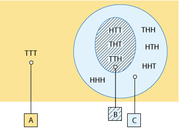
From this visual representation of the events, it is easy to see that event B is totally included in event C, in the sense that every outcome in event B is also an outcome in event C. Also, note that event A stands apart from events B and C, in the sense that they have no outcome in common, or no overlap. At this point these are only noteworthy observations, but as you’ll discover later, they are very important ones.

What if we added the new event:

Event D: “Getting a T on the first toss” → THH, THT, TTH, TTT

How would it look if we added event D to the diagram above? (Link to the answer)

Remember, since H and T are equally likely on each toss, and since there are 8 possible outcomes, the probability of each outcome is 1/8.

See if you can answer the following questions using the diagrams and/or the list of outcomes for each event along with what you have learned so far about probability.

Learn By Doing: Tossing a Fair Coin Three Times

If you were able to answer those questions correctly, you likely have a good instinct for calculating probability! Read on to learn how we will apply this knowledge.

If not, we will try to help you develop this skill in this section.

Comment:

• Note that in event C, “Getting at least one head” there is only one possible outcome which is missing, “Getting NO heads” = TTT. We will address this again when we talk about probability rules, in particular the complement rule. At this point, we just want you to think about how these two events are “opposites” in this scenario.

It is VERY important to realize that just because we can list out the possible outcomes, this does not imply that each outcome is equally likely.

This is the (funny) message in the Daily Show clip we provided on the previous page. But let’s think about this again. In that clip, Walter is claiming that since there are two possible outcomes, the probability is 0.5. The two possible outcomes are

• The world will be destroyed due to use of the large hadron collider
• The world will NOT be destroyed due to use of the large hadron collider

Hopefully it is clear that these two outcomes are not equally likely!!

Let’s consider a more common example.

EXAMPLE: Birth Defects

Suppose we randomly select three children and we are interested in the probability that none of the children have any birth defects.

We use the notation D to represent a child was born with a birth defect and N to represent the child born with NO birth defect. We can list the possible outcomes just as we did for the coin toss, they are:

{DDD, NDD, DND, DDN, DNN, NDN, NND, NNN}

Are the events DDD (all three children are born with birth defects) and NNN (none of the children are born with birth defects) equally likely?

It should be reasonable to you that P(NNN) is much larger than P(DDD).

This is because P(N) and P(D) are not equally likely events.

It is rare (certainly not 50%) for a randomly selected child to be born with a birth defect.

Rules of Probability

Now we move on to learning some of the basic rules of probability.

Fortunately, these rules are very intuitive, and as long as they are applied systematically, they will let us solve more complicated problems; in particular, those problems for which our intuition might be inadequate.

Since most of the probabilities you will be asked to find can be calculated using both

• logic and counting

and

• the rules we will be learning,

we give the following advice as a principle.

PRINCIPLE:

If you can calculate a probability using logic and counting you do not NEED a probability rule (although the correct rule can always be applied)

Probability Rule One

Our first rule simply reminds us of the basic property of probability that we’ve already learned.

The probability of an event, which informs us of the likelihood of it occurring, can range anywhere from 0 (indicating that the event will never occur) to 1 (indicating that the event is certain).

Probability Rule One:

• For any event A, 0 ≤ P(A) ≤ 1.

NOTE: One practical use of this rule is that it can be used to identify any probability calculation that comes out to be more than 1 (or less than 0) as incorrect.

Before moving on to the other rules, let’s first look at an example that will provide a context for illustrating the next several rules.

EXAMPLE: Blood Types

As previously discussed, all human blood can be typed as O, A, B or AB.

In addition, the frequency of the occurrence of these blood types varies by ethnic and racial groups.

According to Stanford University’s Blood Center (bloodcenter.stanford.edu), these are the probabilities of human blood types in the United States (the probability for type A has been omitted on purpose):

Motivating question for rule 2: A person in the United States is chosen at random. What is the probability of the person having blood type A?

Answer Our intuition tells us that since the four blood types O, A, B, and AB exhaust all the possibilities, their probabilities together must sum to 1, which is the probability of a “certain” event (a person has one of these 4 blood types for certain).

Since the probabilities of O, B, and AB together sum to 0.44 + 0.1 + 0.04 = 0.58, the probability of type A must be the remaining 0.42 (1 – 0.58 = 0.42):

Probability Rule Two

This example illustrates our second rule, which tells us that the probability of all possible outcomes together must be 1.

Probability Rule Two:

The sum of the probabilities of all possible outcomes is 1.

This is a good place to compare and contrast what we’re doing here with what we learned in the Exploratory Data Analysis (EDA) section.

• Notice that in this problem we are essentially focusing on a single categorical variable: blood type.
• We summarized this variable above, as we summarized single categorical variables in the EDA section, by listing what values the variable takes and how often it takes them.
• In EDA we used percentages, and here we’re using probabilities, but the two convey the same information.
• In the EDA section, we learned that a pie chart provides an appropriate display when a single categorical variable is involved, and similarly we can use it here (using percentages instead of probabilities):

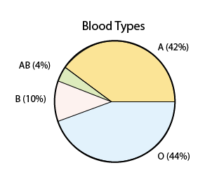
Even though what we’re doing here is indeed similar to what we’ve done in the EDA section, there is a subtle but important difference between the underlying situations

• In EDA, we summarized data that were obtained from a sampleof individuals for whom values of the variable of interest were recorded.
• Here, when we present the probability of each blood type, we have in mind the entire populationof people in the United States, for which we are presuming to know the overall frequency of values taken by the variable of interest.

Did I Get This?: Probability Rule Two

Probability Rule Three

In probability and in its applications, we are frequently interested in finding out the probability that a certain event will not occur.

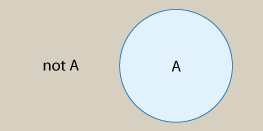
An important point to understand here is that “event A does not occur” is a separate event that consists of all the possible outcomes that are not in A and is called “the complement event of A.”

Notation: we will write “not A” to denote the event that A does not occur. Here is a visual representation of how event A and its complement event “not A” together represent all possible outcomes.

Comment:

• Such a visual display is called a “Venn diagram.” A Venn diagram is a simple way to visualize events and the relationships between them using rectangles and circles.

Rule 3 deals with the relationship between the probability of an event and the probability of its complement event.

Given that event A and event “not A” together make up all possible outcomes, and since rule 2 tells us that the sum of the probabilities of all possible outcomes is 1, the following rule should be quite intuitive:

Probability Rule Three (The Complement Rule):

• P(not A) = 1 – P(A)
• that is, the probability that an event does not occur is 1 minus the probability that it does occur.

EXAMPLE: Blood Types

Back to the blood type example:

Here is some additional information:

• A person with type A can donate blood to a person with type A or AB.
• A person with type B can donate blood to a person with type B or AB.
• A person with type AB can donate blood to a person with type AB only.
• A person with type O blood can donate to anyone.

What is the probability that a randomly chosen person cannot donate blood to everyone? In other words, what is the probability that a randomly chosen person does not have blood type O? We need to find P(not O). Using the Complement Rule, P(not O) = 1 – P(O) = 1 – 0.44 = 0.56. In other words, 56% of the U.S. population does not have blood type O:

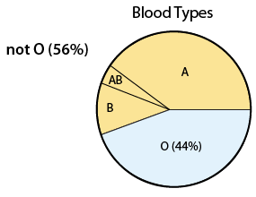
Clearly, we could also find P(not O) directly by adding the probabilities of B, AB, and A.

Comment:

• Note that the Complement Rule, P(not A) = 1 – P(A) can be re-formulated as P(A) = 1 – P(not A).
  • P(not A) = 1 – P(A)
  • can be re-formulated as P(A) = 1 – P(not A).
  • This seemingly trivial algebraic manipulation has an important application, and actually captures the strength of the complement rule.
  • In some cases, when finding P(A) directly is very complicated, it might be much easier to find P(not A) and then just subtract it from 1 to get the desired P(A).
  • We will come back to this comment soon and provide additional examples.

Did I Get This?: Probability Rule Three

Comments:

• The complement rule can be useful whenever it is easier to calculate the probability of the complement of the event rather than the event itself.

• Notice, we again used the phrase “at least one.”
• Now we have seen that the complement of “at least one …” is “none … ” or “no ….” (as we mentioned previously in terms of the events being “opposites”).
• In the above activity we see that
  • P(NONE of these two side effects) = 1 – P(at least one of these two side effects )
• This is a common application of the complement rule which you can often recognize by the phrase “at least one” in the problem.

Probabilities Involving Multiple Events

We will often be interested in finding probabilities involving multiple events such as

• P(A or B) = P(event A occurs or event B occurs or both occur)
• P(A and B)= P(both event A occurs and event B occurs)

A common issue with terminology relates to how we usually think of “or” in our daily life. For example, when a parent says to his or her child in a toy store “Do you want toy A or toy B?”, this means that the child is going to get only one toy and he or she has to choose between them. Getting both toys is usually not an option.

In contrast:

In probability, “OR” means either one or the other or both.

and so P(A or B) = P(event A occurs or event B occurs or BOTH occur)

Having said that, it should be noted that there are some cases where it is simply impossible for the two events to both occur at the same time.

Probability Rule Four

The distinction between events that can happen together and those that cannot is an important one.

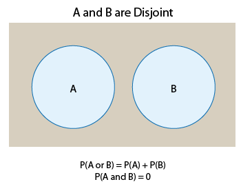
Disjoint: Two events that cannot occur at the same time are called disjoint or mutually exclusive. (We will use disjoint.)

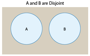
It should be clear from the picture that

• in the first case, where the events are NOT disjoint, P(A and B) ≠ 0
• in the second case, where the events ARE disjoint, P(A and B) = 0.

Here are two examples:

EXAMPLE:

Consider the following two events:

A — a randomly chosen person has blood type A, and

B — a randomly chosen person has blood type B.

In rare cases, it is possible for a person to have more than one type of blood flowing through his or her veins, but for our purposes, we are going to assume that each person can have only one blood type. Therefore, it is impossible for the events A and B to occur together.

• Events A and B are DISJOINT

On the other hand …

EXAMPLE:

Consider the following two events:

A — a randomly chosen person has blood type A

B — a randomly chosen person is a woman.

In this case, it is possible for events A and B to occur together.

• Events A and B are NOT DISJOINT.

The Venn diagrams suggest that another way to think about disjoint versus not disjoint events is that disjoint events do not overlap. They do not share any of the possible outcomes, and therefore cannot happen together.

On the other hand, events that are not disjoint are overlapping in the sense that they share some of the possible outcomes and therefore can occur at the same time.

We now begin with a simple rule for finding P(A or B) for disjoint events.

Probability Rule Four (The Addition Rule for Disjoint Events):

• If A and B are disjoint events, then P(A or B) = P(A) + P(B).

Comment:

• When dealing with probabilities, the word “or” will always be associated with the operation of addition; hence the name of this rule, “The Addition Rule.”

EXAMPLE: Blood Types

Recall the blood type example:

Here is some additional information

• A person with type Acan donate blood to a person with type A or AB.
• A person with type Bcan donate blood to a person with type B or AB.
• A person with type ABcan donate blood to a person with type AB
• A person with type Oblood can donate to anyone.

What is the probability that a randomly chosen person is a potential donor for a person with blood type A?

From the information given, we know that being a potential donor for a person with blood type A means having blood type A or O.

We therefore need to find P(A or O). Since the events A and O are disjoint, we can use the addition rule for disjoint events to get:

• P(A or O) = P(A) + P(O) = 0.42 + 0.44 = 0.86.

It is easy to see why adding the probability actually makes sense.

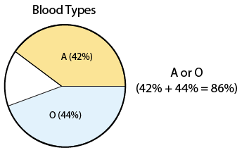
If 42% of the population has blood type A and 44% of the population has blood type O,

• then 42% + 44% = 86% of the population has either blood type A or O, and thus are potential donors to a person with blood type A.

This reasoning about why the addition rule makes sense can be visualized using the pie chart below:

Learn By Doing: Probability Rule Four

Comment:

• The Addition Rule for Disjoint Events can naturally be extended to more than two disjoint events. Let’s take three, for example. If A, B and C are three disjoint events

then P(A or B or C) = P(A) + P(B) + P(C). The rule is the same for any number of disjoint events.

Did I Get This?: Probability Rule Four

We are now finished with the first version of the Addition Rule (Rule four) which is the version restricted to disjoint events. Before covering the second version, we must first discuss P(A and B).

Finding P(A and B) using Logic

We now turn to calculating

• P(A and B)= P(both event A occurs and event B occurs)

Later, we will discuss the rules for calculating P(A and B).

First, we want to illustrate that a rule is not needed whenever you can determine the answer through logic and counting.

Special Case:

There is one special case for which we know what P(A and B) equals without applying any rule.

Learn by Doing: Finding P(A and B) #1

So, if events A and B are disjoint, then (by definition) P(A and B)= 0. But what if the events are not disjoint?

Recall that rule 4, the Addition Rule, has two versions. One is restricted to disjoint events, which we’ve already covered, and we’ll deal with the more general version later in this module. The same will be true of probabilities involving AND

However, except in special cases, we will rely on LOGIC to find P(A and B) in this course.

Before covering any formal rules, let’s look at an example where the events are not disjoint.

EXAMPLE: Periodontal Status and Gender

Learn by Doing: Periodontal Status and Gender

We like to ask probability questions similar to the previous example (using a two-way table based upon data) as this allows you to make connections between these topics and helps you keep some of what you have learned about data fresh in your mind.

Caution

Remember, our primary goal in this course is to analyze real-life data!

Probability Rule Five

We are now ready to move on to the extended version of the Addition Rule.

In this section, we will learn how to find P(A or B) when A and B are not necessarily disjoint.

• We’ll call this extended version the “General Addition Rule” and state it as Probability Rule Five.

We will begin by stating the rule and providing an example similar to the types of problems we generally ask in this course. Then we will present a more another example where we do not have the raw data from a sample to work from.

As we witnessed in previous examples, when the two events are not disjoint, there is some overlap between the events.

• If we simply add the two probabilities together, we will get the wrong answer because we have counted some “probability” twice!
• Thus, we must subtract out this “extra” probability to arrive at the correct answer. The Venn diagram and the two-way tables are helpful in visualizing this idea.

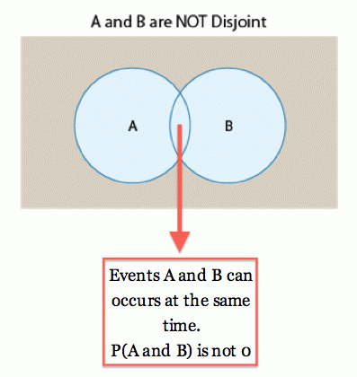
This rule is more general since it works for any pair of events (even disjoint events). Our advice is still to try to answer the question using logic and counting whenever possible, otherwise, we must be extremely careful to choose the correct rule for the problem.

PRINCIPLE:

If you can calculate a probability using logic and counting you do not NEED a probability rule (although the correct rule can always be applied)

Notice that, if A and B are disjoint, then P(A and B) = 0 and rule 5 reduces to rule 4 for this special case.

Let’s revisit the last example:

EXAMPLE: Periodontal Status and Gender

Consider randomly selecting one individual from those represented in the following table regarding the periodontal status of individuals and their gender. Periodontal status refers to gum disease where individuals are classified as either healthy, have gingivitis, or have periodontal disease.

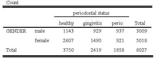
Let’s review what we have learned so far. We can calculate any probability in this scenario if we can determine how many individuals satisfy the event or combination of events.

• P(Male) = 3009/8027 = 0.3749
• P(Female) = 5018/8027 = 0.6251
• P(Healthy) = 3750/8027 = 0.4672
• P(Not Healthy) = P(Gingivitis or Perio) = (2419 + 1858)/8027 = 4277/8027 = 0.5328
  We could also, calculate this using the complement rule: 1 – P(Healthy)

We also previously found that

• P(Male AND Healthy) = 1143/8027 = 0.1424

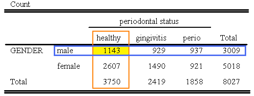
Recall rule 5, P(A or B) = P(A) + P(B) – P(A and B). We now use this rule to calculate P(Male OR Healthy)

• P(Male or Healthy) = P(Male) + P(Healthy) – P(Male and Healthy) = 0.3749 + 0.4672 – 0.1424 = 0.6997 or about 70%

We solved this question earlier by simply counting how many individuals are either Male or Healthy or both. The picture below illustrates the values we need to combine. We need to count

• All males
• All healthy individuals
• BUT, not count anyone twice!!

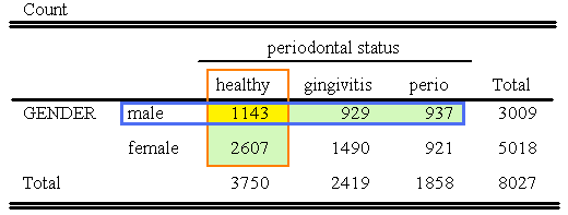
Using this logical approach we would find

• P(Male or Healthy) = (1143 + 929 + 937 + 2607)/8027 = 5616/8027 = 0.6996

We have a minor difference in our answers in the last decimal place due the rounding that occurred when we calculated P(Male), P(Healthy), and P(Male and Healthy) and then applied rule 5.

Clearly the answer is effectively the same, about 70%. If we carried our answers to more decimal places or if we used the original fractions, we could eliminate this small discrepancy entirely.

Let’s look at one final example to illustrate Probability Rule 5 when the rule is needed – i.e. when we don’t have actual data.

EXAMPLE: Important Delivery!

It is vital that a certain document reach its destination within one day. To maximize the chances of on-time delivery, two copies of the document are sent using two services, service A and service B. It is known that the probabilities of on-time delivery are:

• 0.90 for service A (P(A) = 0.90)
• 0.80 for service B (P(B) = 0.80)
• 0.75 for both services being on time (P(A and B) = 0.75)
  (Note that A and B are not disjoint. They can happen together with probability 0.75.)

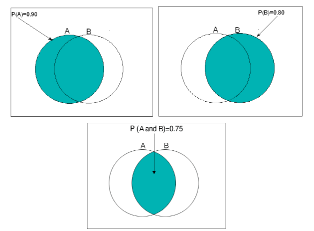
The Venn diagrams below illustrate the probabilities P(A), P(B), and P(A and B) [not drawn to scale]:

In the context of this problem, the obvious question of interest is:

• What is the probability of on-time delivery of the document using this strategy (of sending it via both services)?

The document will reach its destination on time as long as it is delivered on time by service A or by service B or by both services. In other words, when event A occurs or event B occurs or both occur. so….

P(on time delivery using this strategy)= P(A or B), which is represented the by the shaded region in the diagram below:

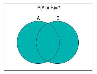
We can now

• use the three Venn diagrams representing P(A), P(B) and P(A and B)
• to see that we can find P(A or B) by adding P(A) (represented by the left circle) and P(B) (represented by the right circle),
• then subtracting P(A and B) (represented by the overlap), since we included it twice, once as part of P(A) and once as part of P(B).

This is shown in the following image:

If we apply this to our example, we find that:

• P(A or B)= P(on-time delivery using this strategy)= 0.90 + 0.80 – 0.75 = 0.95.

So our strategy of using two delivery services increases our probability of on-time delivery to 0.95.

While the Venn diagrams were great to visualize the General Addition Rule, in cases like these it is much easier to display the information in and work with a two-way table of probabilities, much as we examined the relationship between two categorical variables in the Exploratory Data Analysis section.

We will simply show you the table, not how we derive it as you won’t be asked to do this for us. You should be able to see that some logic and simple addition/subtraction is all we used to fill in the table below.

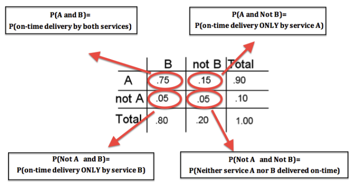
When using a two-way table, we must remember to look at the entire row or column to find overall probabilities involving only A or only B.

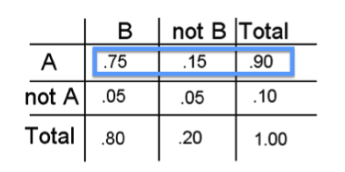
• P(A) = 0.90 means that in 90% of the cases when service A is used, it delivers the document on time. To find this we look at the total probability for the row containing A. In finding P(A), we do not know whether B happens or not.

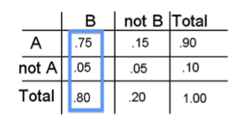
• P(B) = 0.80 means that in 80% of the cases when service B is used, it delivers the document on time. To find this we look at the total probability for the column containing B. In finding P(B), we do not know whether A happens or not.

Comment

• When we used two-way tables in the Exploratory Data Analysis (EDA) section, it was to record values of two categorical variables for a concrete sample of individuals.
• In contrast, the information in a probability two-way table is for an entire population, and the values are rather abstract.
• If we had treated something like the delivery example in the EDA section, we would have recorded the actual numbers of on-time (and not-on-time) deliveries for samples of documents mailed with service A or B.
• In this section, the long-term probabilities are presented as being known.
• Presumably, the reported probabilities in this delivery example were based on relative frequencies recorded over many repetitions.

Interactive Applet: Probability Venn Diagram

Rounding Rule of Thumb for Probability:

Follow the following general guidelines in this course. If in doubt carry more decimal places. If we specify give exactly what is requested.

• In general you should carry probabilities to at least 4 decimal places for intermediate steps.
• We often round our final answer to two or three decimal places.
• For extremely small probabilities, it is important to have 1 or two significant digits (non-zero digits), such as 0.000001 or 0.000034, etc.

Many computer packages might display extremely small values using scientific notation such as

• 58×10^-5 or 1.58 E^-5 to represent 0.0000158

Let’s Summarize

So far in our study of probability, you have been introduced to the sometimes counter-intuitive nature of probability and the fundamentals that underlie probability, such as a relative frequency.

We also gave you some tools to help you find the probabilities of events — namely the probability rules.

You probably noticed that the probability section was significantly different from the two previous sections; it has a much larger technical/mathematical component, so the results tend to be more of the “right or wrong” nature.

In the Exploratory Data Analysis section, for the most part, the computer took care of the technical aspect of things, and our tasks were to tell it to do the right thing and then interpret the results.

In probability, we do the work from beginning to end, from choosing the right tool (rule) to use, to using it correctly, to interpreting the results.

Here is a summary of the rules we have presented so far.

1. Probability Rule #1 states:

• For any event A, 0 ≤ P(A) ≤ 1

2. Probability Rule #2 states:

• The sum of the probabilities of all possible outcomes is 1

3. The Complement Rule (#3) states that

• P(not A) = 1 – P(A)

or when rearranged

• P(A) = 1 – P(not A)

The latter representation of the Complement Rule is especially useful when we need to find probabilities of events of the sort “at least one of …”

4. The General Addition Rule (#5) states that for any two events,

• P(A or B) = P(A) + P(B) – P(A and B),

where, by P(A or B) we mean P(A occurs or B occurs or both).

In the special case of disjoint events, events that cannot occur together, the General Addition Rule can be reduced to the Addition Rule for Disjoint Events (#4), which is

• P(A or B) = P(A) + P(B). *

*ONLY use when you are CONVINCED the events are disjoint (they do NOT overlap)

5. The restricted version of the addition rule (for disjoint events) can be easily extended to more than two events.

6. So far, we have only found P(A and B) using logic and counting in simple examples