Unit 2: Producing Data

Review of the Big Picture

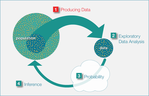
Recall “The Big Picture,” the four-step process that encompasses statistics: data production, exploratory data analysis, probability, and inference.

In the previous unit, we considered exploratory data analysis — the discovery of patterns in the raw data. In this unit, we go back and examine the first step in the process: the production of data. This unit has two main topics; sampling and study design.

Introduction to Producing Data

In the first step of the statistics “Big Picture,” we produce data. The production of data has two stages.

• First we need to choose the individuals from the population that will be included in the sample.
• Then, once we have chosen the individuals, we need to collect data from them.

The first stage is called sampling, and the second stage is called study design.

As we have seen, exploratory data analysis seeks to illuminate patterns in the data by summarizing the distributions of quantitative or categorical variables, or the relationships between variables.

In the final part of the course, statistical inference, we will use the summaries about variables or relationships that were obtained in the study to draw conclusions about what is true for the entire population from which the sample was chosen.

For this process to “work” reliably, it is essential that the sample be truly representative of the larger population. For example, if researchers want to determine whether the antidepressant Zoloft is effective for teenagers in general, then it would not be a good idea to only test it on a sample of teens who have been admitted to a psychiatric hospital, because their depression may be more severe, and less treatable, than that of teens in general.

Thus, the very first stage in data production, sampling, must be carried out in such a way that the sample really does represent the population of interest.

Choosing a sample is only the first stage in producing data, so it is not enough to just make sure that the sample is representative. We must also remember that our summaries of variables and their relationships are only valid if these have been assessed properly.

For instance, if researchers want to test the effectiveness of Zoloft versus Prozac for treating teenagers, it would not be a good idea to simply compare levels of depression for a group of teenagers who happen to be using Zoloft to levels of depression for a group of teenagers who happen to be using Prozac. If they discover that one group of patients turns out to be less depressed, it could just be that teenagers with less serious depression are more likely to be prescribed one of the drugs over the other.

In situations like this, the design for producing data must be considered carefully. Studies should be designed to discover what we want to know about the variables of interest for the individuals in the sample.

In particular, if what you want to know about the variables is whether there is a causal relationship between them, special care should be given to the design of the study (since, as we know, association does not imply causation).

In this unit, we will focus on these two stages of data production: obtaining a sample, and designing a study.

Throughout this unit, we establish guidelines for the ideal production of data. While we will hold these guidelines as standards to strive for, realistically it is rarely possible to carry out a study that is completely free of flaws. Common sense must frequently be applied in order to decide which imperfections we can live with and which ones could completely undermine a study’s results.

A sample that produces data that is not representative because of the systematic under- or over-estimation of the values of the variable of interest is called biased. Bias may result from either a poor sampling plan or from a poor design for evaluating the variable of interest.

We begin this unit by focusing on what constitutes a good — or a bad — sampling plan after which we will discuss study design.