
3.2: Measures of Central Tendency
- Page ID
- 7093

\( \newcommand{\vecs}[1]{\overset { \scriptstyle \rightharpoonup} {\mathbf{#1}} } \)
\( \newcommand{\vecd}[1]{\overset{-\!-\!\rightharpoonup}{\vphantom{a}\smash {#1}}} \)
\( \newcommand{\id}{\mathrm{id}}\) \( \newcommand{\Span}{\mathrm{span}}\)
( \newcommand{\kernel}{\mathrm{null}\,}\) \( \newcommand{\range}{\mathrm{range}\,}\)
\( \newcommand{\RealPart}{\mathrm{Re}}\) \( \newcommand{\ImaginaryPart}{\mathrm{Im}}\)
\( \newcommand{\Argument}{\mathrm{Arg}}\) \( \newcommand{\norm}[1]{\| #1 \|}\)
\( \newcommand{\inner}[2]{\langle #1, #2 \rangle}\)
\( \newcommand{\Span}{\mathrm{span}}\)
\( \newcommand{\id}{\mathrm{id}}\)
\( \newcommand{\Span}{\mathrm{span}}\)
\( \newcommand{\kernel}{\mathrm{null}\,}\)
\( \newcommand{\range}{\mathrm{range}\,}\)
\( \newcommand{\RealPart}{\mathrm{Re}}\)
\( \newcommand{\ImaginaryPart}{\mathrm{Im}}\)
\( \newcommand{\Argument}{\mathrm{Arg}}\)
\( \newcommand{\norm}[1]{\| #1 \|}\)
\( \newcommand{\inner}[2]{\langle #1, #2 \rangle}\)
\( \newcommand{\Span}{\mathrm{span}}\) \( \newcommand{\AA}{\unicode[.8,0]{x212B}}\)
\( \newcommand{\vectorA}[1]{\vec{#1}} % arrow\)
\( \newcommand{\vectorAt}[1]{\vec{\text{#1}}} % arrow\)
\( \newcommand{\vectorB}[1]{\overset { \scriptstyle \rightharpoonup} {\mathbf{#1}} } \)
\( \newcommand{\vectorC}[1]{\textbf{#1}} \)
\( \newcommand{\vectorD}[1]{\overrightarrow{#1}} \)
\( \newcommand{\vectorDt}[1]{\overrightarrow{\text{#1}}} \)
\( \newcommand{\vectE}[1]{\overset{-\!-\!\rightharpoonup}{\vphantom{a}\smash{\mathbf {#1}}}} \)
\( \newcommand{\vecs}[1]{\overset { \scriptstyle \rightharpoonup} {\mathbf{#1}} } \)
\( \newcommand{\vecd}[1]{\overset{-\!-\!\rightharpoonup}{\vphantom{a}\smash {#1}}} \)
\(\newcommand{\avec}{\mathbf a}\) \(\newcommand{\bvec}{\mathbf b}\) \(\newcommand{\cvec}{\mathbf c}\) \(\newcommand{\dvec}{\mathbf d}\) \(\newcommand{\dtil}{\widetilde{\mathbf d}}\) \(\newcommand{\evec}{\mathbf e}\) \(\newcommand{\fvec}{\mathbf f}\) \(\newcommand{\nvec}{\mathbf n}\) \(\newcommand{\pvec}{\mathbf p}\) \(\newcommand{\qvec}{\mathbf q}\) \(\newcommand{\svec}{\mathbf s}\) \(\newcommand{\tvec}{\mathbf t}\) \(\newcommand{\uvec}{\mathbf u}\) \(\newcommand{\vvec}{\mathbf v}\) \(\newcommand{\wvec}{\mathbf w}\) \(\newcommand{\xvec}{\mathbf x}\) \(\newcommand{\yvec}{\mathbf y}\) \(\newcommand{\zvec}{\mathbf z}\) \(\newcommand{\rvec}{\mathbf r}\) \(\newcommand{\mvec}{\mathbf m}\) \(\newcommand{\zerovec}{\mathbf 0}\) \(\newcommand{\onevec}{\mathbf 1}\) \(\newcommand{\real}{\mathbb R}\) \(\newcommand{\twovec}[2]{\left[\begin{array}{r}#1 \\ #2 \end{array}\right]}\) \(\newcommand{\ctwovec}[2]{\left[\begin{array}{c}#1 \\ #2 \end{array}\right]}\) \(\newcommand{\threevec}[3]{\left[\begin{array}{r}#1 \\ #2 \\ #3 \end{array}\right]}\) \(\newcommand{\cthreevec}[3]{\left[\begin{array}{c}#1 \\ #2 \\ #3 \end{array}\right]}\) \(\newcommand{\fourvec}[4]{\left[\begin{array}{r}#1 \\ #2 \\ #3 \\ #4 \end{array}\right]}\) \(\newcommand{\cfourvec}[4]{\left[\begin{array}{c}#1 \\ #2 \\ #3 \\ #4 \end{array}\right]}\) \(\newcommand{\fivevec}[5]{\left[\begin{array}{r}#1 \\ #2 \\ #3 \\ #4 \\ #5 \\ \end{array}\right]}\) \(\newcommand{\cfivevec}[5]{\left[\begin{array}{c}#1 \\ #2 \\ #3 \\ #4 \\ #5 \\ \end{array}\right]}\) \(\newcommand{\mattwo}[4]{\left[\begin{array}{rr}#1 \amp #2 \\ #3 \amp #4 \\ \end{array}\right]}\) \(\newcommand{\laspan}[1]{\text{Span}\{#1\}}\) \(\newcommand{\bcal}{\cal B}\) \(\newcommand{\ccal}{\cal C}\) \(\newcommand{\scal}{\cal S}\) \(\newcommand{\wcal}{\cal W}\) \(\newcommand{\ecal}{\cal E}\) \(\newcommand{\coords}[2]{\left\{#1\right\}_{#2}}\) \(\newcommand{\gray}[1]{\color{gray}{#1}}\) \(\newcommand{\lgray}[1]{\color{lightgray}{#1}}\) \(\newcommand{\rank}{\operatorname{rank}}\) \(\newcommand{\row}{\text{Row}}\) \(\newcommand{\col}{\text{Col}}\) \(\renewcommand{\row}{\text{Row}}\) \(\newcommand{\nul}{\text{Nul}}\) \(\newcommand{\var}{\text{Var}}\) \(\newcommand{\corr}{\text{corr}}\) \(\newcommand{\len}[1]{\left|#1\right|}\) \(\newcommand{\bbar}{\overline{\bvec}}\) \(\newcommand{\bhat}{\widehat{\bvec}}\) \(\newcommand{\bperp}{\bvec^\perp}\) \(\newcommand{\xhat}{\widehat{\xvec}}\) \(\newcommand{\vhat}{\widehat{\vvec}}\) \(\newcommand{\uhat}{\widehat{\uvec}}\) \(\newcommand{\what}{\widehat{\wvec}}\) \(\newcommand{\Sighat}{\widehat{\Sigma}}\) \(\newcommand{\lt}{<}\) \(\newcommand{\gt}{>}\) \(\newcommand{\amp}{&}\) \(\definecolor{fillinmathshade}{gray}{0.9}\)In the previous section we saw that there are several ways to define central tendency. This section defines the three most common measures of central tendency: the mean, the median, and the mode. The relationships among these measures of central tendency and the definitions given in the previous section will probably not be obvious to you.
This section gives only the basic definitions of the mean, median and mode. A further discussion of the relative merits and proper applications of these statistics is presented in a later section.
Arithmetic Mean
The arithmetic mean is the most common measure of central tendency. It is simply the sum of the numbers divided by the number of numbers. The symbol “\(\mu \)” (pronounced “mew”) is used for the mean of a population. The symbol “\(\overline{\mathrm{X}}\)” (pronounced “X-bar”) is used for the mean of a sample. The formula for \(\mu \) is shown below:
\[\mu=\dfrac{\sum \mathrm{X}}{N}\]
where \(\Sigma \mathbf{X} \) is the sum of all the numbers in the population and \(N\) is the number of numbers in the population.
The formula for \(\overline{\mathrm{X}} \) is essentially identical:
\[\overline{\mathrm{X}}=\dfrac{\sum \mathrm{X}}{N} \]
where \(\Sigma \mathbf{X} \) is the sum of all the numbers in the sample and \(N\) is the number of numbers in the sample. The only distinction between these two equations is whether we are referring to the population (in which case we use the parameter \(\mu \)) or a sample of that population (in which case we use the statistic \(\overline{\mathrm{X}}\)).
As an example, the mean of the numbers 1, 2, 3, 6, 8 is 20/5 = 4 regardless of whether the numbers constitute the entire population or just a sample from the population.
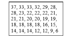
Figure \(\PageIndex{1}\) shows the number of touchdown (TD) passes thrown by each of the 31 teams in the National Football League in the 2000 season. The mean number of touchdown passes thrown is 20.45 as shown below.
\[\mu=\dfrac{\sum X}{N}=\dfrac{634}{31}=20.45 \nonumber \]
Although the arithmetic mean is not the only “mean” (there is also a geometric mean, a harmonic mean, and many others that are all beyond the scope of this course), it is by far the most commonly used. Therefore, if the term “mean” is used without specifying whether it is the arithmetic mean, the geometric mean, or some other mean, it is assumed to refer to the arithmetic mean.
Median The median is also a frequently used measure of central tendency. The median is the midpoint of a distribution: the same number of scores is above the median as below it. For the data in Figure \(\PageIndex{1}\), there are 31 scores. The 16th highest score (which equals 20) is the median because there are 15 scores below the 16th score and 15 scores above the 16th score. The median can also be thought of as the 50th percentile.
When there is an odd number of numbers, the median is simply the middle number. For example, the median of 2, 4, and 7 is 4. When there is an even number of numbers, the median is the mean of the two middle numbers. Thus, the median of the numbers 2, 4, 7, 12 is:
\[\dfrac{4+7}{2}=5.5 \nonumber \]
When there are numbers with the same values, each appearance of that value gets counted. For example, in the set of numbers 1, 3, 4, 4, 5, 8, and 9, the median is 4 because there are three numbers (1, 3, and 4) below it and three numbers (5, 8, and 9) above it. If we only counted 4 once, the median would incorrectly be calculated at 4.5 (4+5 divided by 2). When in doubt, writing out all of the numbers in order and marking them off one at a time from the top and bottom will always lead you to the correct answer.
Mode
The mode is the most frequently occurring value in the dataset. For the data in Figure \(\PageIndex{1}\), the mode is 18 since more teams (4) had 18 touchdown passes than any other number of touchdown passes. With continuous data, such as response time measured to many decimals, the frequency of each value is one since no two scores will be exactly the same (see discussion of continuous variables). Therefore the mode of continuous data is normally computed from a grouped frequency distribution. Table \(\PageIndex{1}\) shows a grouped frequency distribution for the target response time data. Since the interval with the highest frequency is 600-700, the mode is the middle of that interval (650). Though the mode is not frequently used for continuous data, it is nevertheless an important measure of central tendency as it is the only measure we can use on qualitative or categorical data.
| Range | Frequency |
|---|---|
| 500 - 600 | 3 |
| 600 - 700 | 6 |
| 700 - 800 | 5 |
| 800 - 900 | 5 |
| 900 - 1000 | 0 |
| 1000 - 1100 | 1 |
More on the Mean and Median
In the section “What is central tendency,” we saw that the center of a distribution could be defined three ways:
- the point on which a distribution would balance
- the value whose average absolute deviation from all the other values is minimized
- the value whose squared difference from all the other values is minimized.
The mean is the point on which a distribution would balance, the median is the value that minimizes the sum of absolute deviations, and the mean is the value that minimizes the sum of the squared deviations.
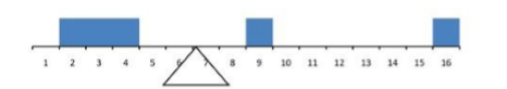
Table \(\PageIndex{2}\) shows the absolute and squared deviations of the numbers 2, 3, 4, 9, and 16 from their median of 4 and their mean of 6.8. You can see that the sum of absolute deviations from the median (20) is smaller than the sum of absolute deviations from the mean (22.8). On the other hand, the sum of squared deviations from the median (174) is larger than the sum of squared deviations from the mean (134.8).
| Value | Absolute Deviation from Median | Absolute Deviation from Mean | Squared Deviation from Median | Squared Deviation from Mean |
|---|---|---|---|---|
| 2 | 2 | 4.8 | 4 | 23.04 |
| 3 | 1 | 3.8 | 1 | 14.44 |
| 4 | 0 | 2.8 | 0 | 7.84 |
| 9 | 5 | 2.2 | 25 | 4.84 |
| 16 | 12 | 9.2 | 144 | 84.64 |
| Total | 20 | 22.8 | 174 | 134.8 |
Figure \(\PageIndex{2}\) shows that the distribution balances at the mean of 6.8 and not at the median of 4. The relative advantages and disadvantages of the mean and median are discussed in the section “Comparing Measures” later in this chapter.
When a distribution is symmetric, then the mean and the median are the same. Consider the following distribution: 1, 3, 4, 5, 6, 7, 9. The mean and median are both 5. The mean, median, and mode are identical in the bell-shaped normal distribution.
Comparing Measures of Central Tendency
How do the various measures of central tendency compare with each other? For symmetric distributions, the mean and median, as is the mode except in bimodal distributions. Differences among the measures occur with skewed distributions. Figure \(\PageIndex{3}\) shows the distribution of 642 scores on an introductory psychology test. Notice this distribution has a slight positive skew.
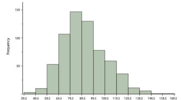
Measures of central tendency are shown in Table \(\PageIndex{3}\). Notice they do not differ greatly, with the exception that the mode is considerably lower than the other measures. When distributions have a positive skew, the mean is typically higher than the median, although it may not be in bimodal distributions. For these data, the mean of 91.58 is higher than the median of 90. This pattern holds true for any skew: the mode will remain at the highest point in the distribution, the median will be pulled slightly out into the skewed tail (the longer end of the distribution), and the mean will be pulled the farthest out. Thus, the mean is more sensitive to skew than the median or mode, and in cases of extreme skew, the mean may no longer be appropriate to use.
| Measure | Value |
|---|---|
| Mode | 84.00 |
| Median | 90.00 |
| Mean | 91.58 |
The distribution of baseball salaries (in 1994) shown in Figure \(\PageIndex{4}\) has a much more pronounced skew than the distribution in Figure \(\PageIndex{3}\).
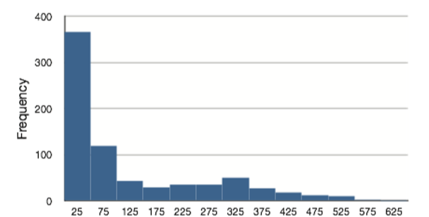
Table \(\PageIndex{4}\) shows the measures of central tendency for these data. The large skew results in very different values for these measures. No single measure of central tendency is sufficient for data such as these. If you were asked the very general question: “So, what do baseball players make?” and answered with the mean of $1,183,000, you would not have told the whole story since only about one third of baseball players make that much. If you answered with the mode of $250,000 or the median of $500,000, you would not be giving any indication that some players make many millions of dollars. Fortunately, there is no need to summarize a distribution with a single number. When the various measures differ, our opinion is that you should report the mean and median. Sometimes it is worth reporting the mode as well. In the media, the median is usually reported to summarize the center of skewed distributions. You will hear about median salaries and median prices of houses sold, etc. This is better than reporting only the mean, but it would be informative to hear more statistics.
| Measure | Value |
|---|---|
| Mode | 250 |
| Median | 500 |
| Mean | 1,183 |