3.3: Spread and Variability
- Page ID
- 7094

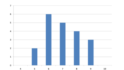
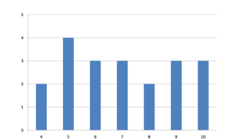
Variability refers to how “spread out” a group of scores is. To see what we mean by spread out, consider graphs in Figure \(\PageIndex{1}\). These graphs represent the scores on two quizzes. The mean score for each quiz is 7.0. Despite the equality of means, you can see that the distributions are quite different. Specifically, the scores on Quiz 1 are more densely packed and those on Quiz 2 are more spread out. The differences among students were much greater on Quiz 2 than on Quiz 1.
The terms variability, spread, and dispersion are synonyms, and refer to how spread out a distribution is. Just as in the section on central tendency where we discussed measures of the center of a distribution of scores, in this chapter we will discuss measures of the variability of a distribution. There are three frequently used measures of variability: range, variance, and standard deviation. In the next few paragraphs, we will look at each of these measures of variability in more detail.
Range
The range is the simplest measure of variability to calculate, and one you have probably encountered many times in your life. The range is simply the highest score minus the lowest score. Let’s take a few examples. What is the range of the following group of numbers: 10, 2, 5, 6, 7, 3, 4? Well, the highest number is 10, and the lowest number is 2, so 10 - 2 = 8. The range is 8. Let’s take another example. Here’s a dataset with 10 numbers: 99, 45, 23, 67, 45, 91, 82, 78, 62, 51. What is the range? The highest number is 99 and the lowest number is 23, so 99 - 23 equals 76; the range is 76. Now consider the two quizzes shown in Figure \(\PageIndex{1}\) and Figure \(\PageIndex{2}\). On Quiz 1, the lowest score is 5 and the highest score is 9. Therefore, the range is 4. The range on Quiz 2 was larger: the lowest score was 4 and the highest score was 10. Therefore the range is 6.
The problem with using range is that it is extremely sensitive to outliers, and one number far away from the rest of the data will greatly alter the value of the range. For example, in the set of numbers 1, 3, 4, 4, 5, 8, and 9, the range is 8 (9 – 1).
However, if we add a single person whose score is nowhere close to the rest of the scores, say, 20, the range more than doubles from 8 to 19.
Interquartile Range
The interquartile range (IQR) is the range of the middle 50% of the scores in a distribution and is sometimes used to communicate where the bulk of the data in the distribution are located. It is computed as follows:
\[\text {IQR} = 75\text {th percentile }- 25\text {th percentile}\]
For Quiz 1, the 75th percentile is 8 and the 25th percentile is 6. The interquartile range is therefore 2. For Quiz 2, which has greater spread, the 75th percentile is 9, the 25th percentile is 5, and the interquartile range is 4. Recall that in the discussion of box plots, the 75th percentile was called the upper hinge and the 25th percentile was called the lower hinge. Using this terminology, the interquartile range is referred to as the H-spread.
Sum of Squares
Variability can also be defined in terms of how close the scores in the distribution are to the middle of the distribution. Using the mean as the measure of the middle of the distribution, we can see how far, on average, each data point is from the center. The data from Quiz 1 are shown in Table \(\PageIndex{1}\). The mean score is 7.0 (\(\Sigma \mathrm{X} / \mathrm{N}= 140/20 = 7\)). Therefore, the column “\(X-\overline {X}\)” contains deviations (how far each score deviates from the mean), here calculated as the score minus 7. The column “\((X-\overline {X})^{2}\)” has the “Squared Deviations” and is simply the previous column squared.
There are a few things to note about how Table \(\PageIndex{1}\) is formatted, as this is the format you will use to calculate variance (and, soon, standard deviation). The raw data scores (\(\mathrm{X}\)) are always placed in the left-most column. This column is then summed at the bottom to facilitate calculating the mean (simply divided this number by the number of scores in the table). Once you have the mean, you can easily work your way down the middle column calculating the deviation scores. This column is also summed and has a very important property: it will always sum to 0 (or close to zero if you have rounding error due to many decimal places). This step is used as a check on your math to make sure you haven’t made a mistake. If this column sums to 0, you can move on to filling in the third column of squared deviations. This column is summed as well and has its own name: the Sum of Squares (abbreviated as \(SS\) and given the formula \(∑(X-\overline {X})^{2}\)). As we will see, the Sum of Squares appears again and again in different formulas – it is a very important value, and this table makes it simple to calculate without error.
| \(\mathrm{X}\) | \(X-\overline{X}\) | \((X-\overline {X})^{2}\) |
|---|---|---|
| 9 | 2 | 4 |
| 9 | 2 | 4 |
| 9 | 2 | 4 |
| 8 | 1 | 1 |
| 8 | 1 | 1 |
| 8 | 1 | 1 |
| 8 | 1 | 1 |
| 7 | 0 | 0 |
| 7 | 0 | 0 |
| 7 | 0 | 0 |
| 7 | 0 | 0 |
| 7 | 0 | 0 |
| 6 | -1 | 1 |
| 6 | -1 | 1 |
| 6 | -1 | 1 |
| 6 | -1 | 1 |
| 6 | -1 | 1 |
| 6 | -1 | 1 |
| 5 | -2 | 4 |
| 5 | -2 | 4 |
| \(\Sigma = 140\) | \(\Sigma = 0\) | \(\Sigma = 30\) |
Variance
Now that we have the Sum of Squares calculated, we can use it to compute our formal measure of average distance from the mean, the variance. The variance is defined as the average squared difference of the scores from the mean. We square the deviation scores because, as we saw in the Sum of Squares table, the sum of raw deviations is always 0, and there’s nothing we can do mathematically without changing that.
The population parameter for variance is \(σ^2\) (“sigma-squared”) and is calculated as:
\[\sigma^{2}=\dfrac{\sum(X-\mu)^{2}}{N} \]
Notice that the numerator that formula is identical to the formula for Sum of Squares presented above with \(\overline {X}\) replaced by \(μ\). Thus, we can use the Sum of Squares table to easily calculate the numerator then simply divide that value by \(N\) to get variance. If we assume that the values in Table \(\PageIndex{1}\) represent the full population, then we can take our value of Sum of Squares and divide it by \(N\) to get our population variance:
\[\sigma^{2}=\dfrac{30}{20}=1.5 \nonumber \]
So, on average, scores in this population are 1.5 squared units away from the mean. This measure of spread is much more robust (a term used by statisticians to mean resilient or resistant to) outliers than the range, so it is a much more useful value to compute. Additionally, as we will see in future chapters, variance plays a central role in inferential statistics.
The sample statistic used to estimate the variance is \(s^2\) (“s-squared”):
\[s^{2}=\dfrac{\sum(X-\overline{X})^{2}}{N-1} \]
This formula is very similar to the formula for the population variance with one change: we now divide by \(N – 1\) instead of \(N\). The value \(N – 1\) has a special name: the degrees of freedom (abbreviated as \(df\)). You don’t need to understand in depth what degrees of freedom are (essentially they account for the fact that we have to use a sample statistic to estimate the mean (\(\overline {X}\)) before we estimate the variance) in order to calculate variance, but knowing that the denominator is called \(df\) provides a nice shorthand for the variance formula: \(SS/df\).
Going back to the values in Table \(\PageIndex{1}\) and treating those scores as a sample, we can estimate the sample variance as:
\[s^{2}=\dfrac{30}{20-1}=1.58 \]
Notice that this value is slightly larger than the one we calculated when we assumed these scores were the full population. This is because our value in the denominator is slightly smaller, making the final value larger. In general, as your sample size \(N\) gets bigger, the effect of subtracting 1 becomes less and less. Comparing a sample size of 10 to a sample size of 1000; 10 – 1 = 9, or 90% of the original value, whereas 1000 – 1 = 999, or 99.9% of the original value. Thus, larger sample sizes will bring the estimate of the sample variance closer to that of the population variance. This is a key idea and principle in statistics that we will see over and over again: larger sample sizes better reflect the population.
Standard Deviation
The standard deviation is simply the square root of the variance. This is a useful and interpretable statistic because taking the square root of the variance (recalling that variance is the average squared difference) puts the standard deviation back into the original units of the measure we used. Thus, when reporting descriptive statistics in a study, scientists virtually always report mean and standard deviation. Standard deviation is therefore the most commonly used measure of spread for our purposes.
The population parameter for standard deviation is \(σ\) (“sigma”), which, intuitively, is the square root of the variance parameter \(σ^2\) (on occasion, the symbols work out nicely that way). The formula is simply the formula for variance under a square root sign:
\[\sigma=\sqrt{\dfrac{\sum(X-\mu)^{2}}{N}} \]
Back to our earlier example from Table \(\PageIndex{1}\):
\[\sigma=\sqrt{\dfrac{30}{20}}=\sqrt{1.5}=1.22 \nonumber \]
The sample statistic follows the same conventions and is given as \(s\):
\[s=\sqrt{\dfrac{\sum(X-\overline {X})^{2}}{N-1}}=\sqrt{\dfrac{S S}{d f}} \]
The sample standard deviation from Table \(\PageIndex{1}\) is:
\[s=\sqrt{\dfrac{30}{20-1}}=\sqrt{1.58}=1.26 \nonumber \]
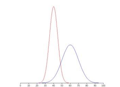
The standard deviation is an especially useful measure of variability when the distribution is normal or approximately normal because the proportion of the distribution within a given number of standard deviations from the mean can be calculated. For example, 68% of the distribution is within one standard deviation (above and below) of the mean and approximately 95% of the distribution is within two standard deviations of the mean. Therefore, if you had a normal distribution with a mean of 50 and a standard deviation of 10, then 68% of the distribution would be between 50 - 10 = 40 and 50 +10 =60. Similarly, about 95% of the distribution would be between 50 - 2 x 10 = 30 and 50 + 2 x 10 = 70.
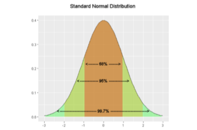
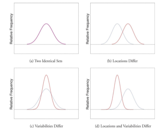
Figure \(\PageIndex{4}\) shows two normal distributions. The red distribution has a mean of 40 and a standard deviation of 5; the blue distribution has a mean of 60 and a standard deviation of 10. For the red distribution, 68% of the distribution is between 45 and 55; for the blue distribution, 68% is between 50 and 70. Notice that as the standard deviation gets smaller, the distribution becomes much narrower, regardless of where the center of the distribution (mean) is. Figure \(\PageIndex{5}\) presents several more examples of this effect.