8.14: Case study - Forced expiratory volume model selection using AICs

Last updated
Save as PDF

Page ID: 33304

\( \newcommand{\vecs}[1]{\overset { \scriptstyle \rightharpoonup} {\mathbf{#1}} } \) \( \newcommand{\vecd}[1]{\overset{-\!-\!\rightharpoonup}{\vphantom{a}\smash {#1}}} \)\(\newcommand{\id}{\mathrm{id}}\) \( \newcommand{\Span}{\mathrm{span}}\) \( \newcommand{\kernel}{\mathrm{null}\,}\) \( \newcommand{\range}{\mathrm{range}\,}\) \( \newcommand{\RealPart}{\mathrm{Re}}\) \( \newcommand{\ImaginaryPart}{\mathrm{Im}}\) \( \newcommand{\Argument}{\mathrm{Arg}}\) \( \newcommand{\norm}[1]{\| #1 \|}\) \( \newcommand{\inner}[2]{\langle #1, #2 \rangle}\) \( \newcommand{\Span}{\mathrm{span}}\) \(\newcommand{\id}{\mathrm{id}}\) \( \newcommand{\Span}{\mathrm{span}}\) \( \newcommand{\kernel}{\mathrm{null}\,}\) \( \newcommand{\range}{\mathrm{range}\,}\) \( \newcommand{\RealPart}{\mathrm{Re}}\) \( \newcommand{\ImaginaryPart}{\mathrm{Im}}\) \( \newcommand{\Argument}{\mathrm{Arg}}\) \( \newcommand{\norm}[1]{\| #1 \|}\) \( \newcommand{\inner}[2]{\langle #1, #2 \rangle}\) \( \newcommand{\Span}{\mathrm{span}}\)\(\newcommand{\AA}{\unicode[.8,0]{x212B}}\)

Researchers were interested in studying the effects of smoking by children on their lung development by measuring the forced expiratory volume (FEV, measured in Liters) in a representative sample of children (\(n = 654\)) between the ages of 3 and 19; this data set is available in the FEV data set in the coneproj package (M. C. Meyer and Liao (2021), Liao and Meyer (2014)). Measurements on the age (in years) and height (in inches) as well as the sex and smoking status of the children were made. We would expect both the age and height to have positive relationships with FEV (lung capacity) and that smoking might decrease the lung capacity but also that older children would be more likely to smoke. So the height and age might be confounded with smoking status and smoking might diminish lung development for older kids – resulting in a potential interaction between age and smoking. The sex of the child might also matter and should be considered or at least controlled for since the response is a size-based measure. This creates the potential for including up to four variables (age, height, sex, and smoking status) and possibly the interaction between age and smoking status. Initial explorations suggested that modeling the log-FEV would be more successful than trying to model the responses on the original scale. Figure 8.42 shows the suggestion of different slopes for the smokers than non-smokers and that there aren’t very many smokers under 9 years old in the data set.

So we will start with a model that contains an age by smoking interaction and include height and sex as additive terms. We are not sure if any of these model components will be needed, so the simplest candidate model will be to remove all the predictors and just have a mean-only model (FEV ~ 1). In between the mean-only and most complicated model are many different options where we can drop the interaction or drop the additive terms or drop the terms involved in the interaction if we don’t need the interaction.

Figure 8.42: Scatterplot of log(FEV) vs Age by smoking status, with both combined (top) and faceted (bottom) versions.

library(coneproj)
data(FEV)
FEV <- as_tibble(FEV)
FEV <- FEV %>% mutate(sex = factor(sex), #Make sex and smoke factors, log.FEV
                      smoke = factor(smoke),
                      log.FEV = log(FEV))
levels(FEV$sex) <- c("Female","Male") #Make sex labels explicit
levels(FEV$smoke) <- c("Nonsmoker","Smoker") #Make smoking status labels explicit

p1 <- FEV %>% ggplot(mapping = aes(x = age, y = log.FEV, color = smoke, shape = smoke)) +
  geom_point(size = 1.5, alpha = 0.5) +
  geom_smooth(method = "lm") +
  theme_bw() +
  scale_color_viridis_d(end = 0.8) +
  labs(title = "Plot of log(FEV) vs Age of children by smoking  status",
       y = "log(FEV)") 

p2 <- FEV %>% ggplot(mapping = aes(x = age, y = log.FEV, color = smoke, shape = smoke)) +
  geom_point(size = 1.5, alpha = 0.5) +
  geom_smooth(method = "lm") +
  theme_bw() +
  scale_color_viridis_d(end = 0.8) +
  labs(title = "Plot of log(FEV) vs Age of children by smoking  status",
       y = "log(FEV)") +
  facet_grid(cols = vars(smoke))

grid.arrange(p1, p2, nrow = 2)

To get the needed results, start with the full model – the most complicated model you want to consider. It is good to check assumptions before considering reducing the model as they rarely get better in simpler models and the AIC is only appropriate to use if the model assumptions are not clearly violated. As suggested above, our “fullish” model for the log(FEV) values is specified as log(FEV) ~ height + age * smoke + sex.

fm1 <- lm(log.FEV ~ height + age * smoke + sex, data = FEV)
summary(fm1)

## 
## Call:
## lm(formula = log.FEV ~ height + age * smoke + sex, data = FEV)
## 
## Residuals:
##      Min       1Q   Median       3Q      Max 
## -0.62926 -0.08783  0.01136  0.09658  0.40751 
## 
## Coefficients:
##                  Estimate Std. Error t value Pr(>|t|)
## (Intercept)     -1.919494   0.080571 -23.824  < 2e-16
## height           0.042066   0.001759  23.911  < 2e-16
## age              0.025368   0.003642   6.966 8.03e-12
## smokeSmoker      0.107884   0.113646   0.949  0.34282
## sexMale          0.030871   0.011764   2.624  0.00889
## age:smokeSmoker -0.011666   0.008465  -1.378  0.16863
## 
## Residual standard error: 0.1454 on 648 degrees of freedom
## Multiple R-squared:  0.8112, Adjusted R-squared:  0.8097 
## F-statistic: 556.8 on 5 and 648 DF,  p-value: < 2.2e-16

par(mfrow = c(2,2), oma = c(0,0,2,0))
plot(fm1, pch = 16, sub.caption = "")
title(main="Diagnostics for full FEV model", outer=TRUE)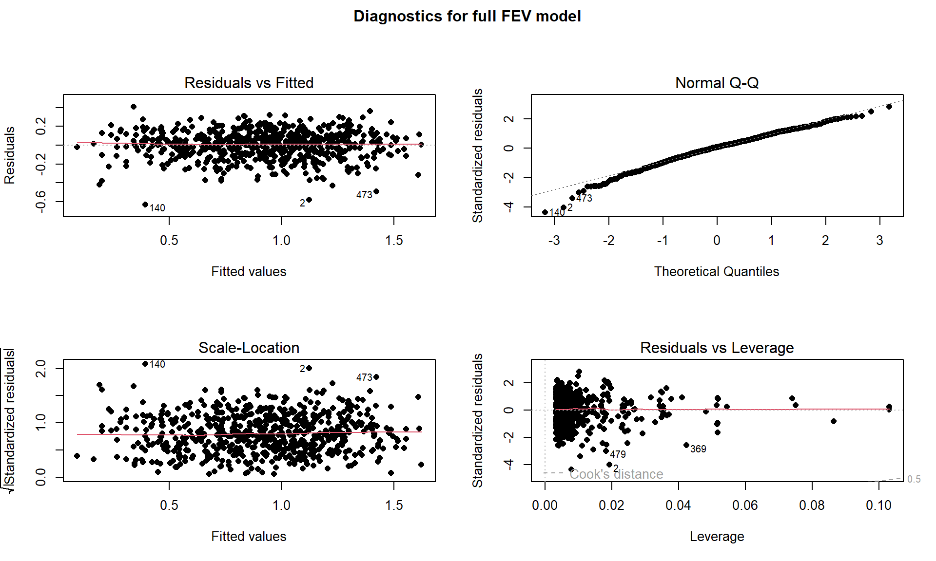

Figure 8.43: Diagnostics for the log(FEV) model that includes height, sex, and an interaction between age and smoking status (the full model).

The diagnostic plots suggest that there are a few outlying points (Figure 8.43) but they are not influential and there is no indication of violations of the constant variance assumption. There is a slight left skew with a long left tail to cause a very minor concern with the normality assumption but not enough to be concerned about our inferences from this model. If we select a different model(s), we would want to check its diagnostics and make sure that the results do not look noticeably worse than these do.

plot(allEffects(fm1, residuals = T), grid = T)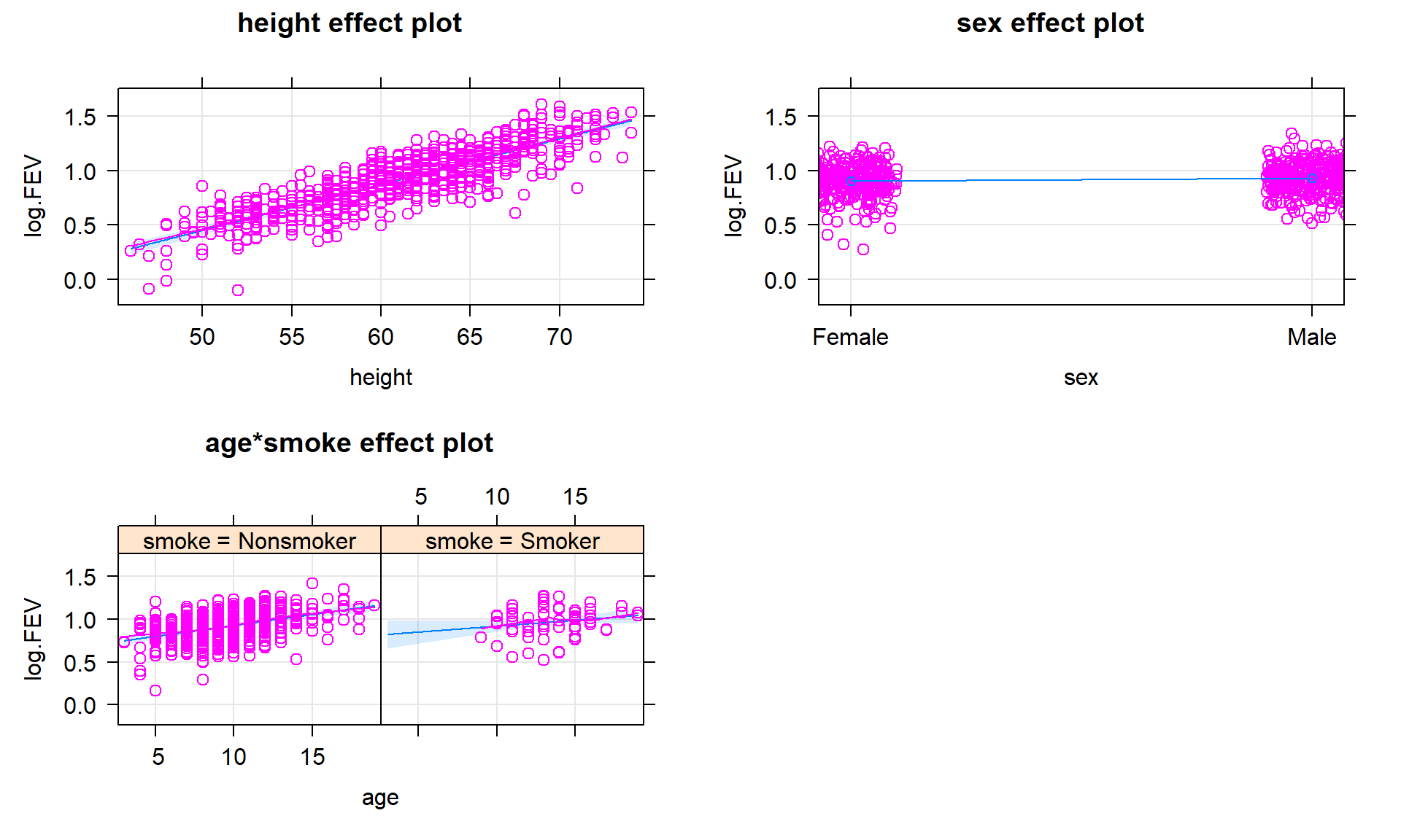

Figure 8.44: Term-plots for the log(FEV) model that includes height, sex, and an interaction between age and smoking status (the full model), with partial residuals.

Figure 8.44 provides our first term-plot with multiple predictors and an interaction. Each term is interpreted using our “conditional” language for any of the other two panels. So we could explore the impacts of height on log-fev after controlling for sex as well as age, smoking status, and the age by smoking interaction. This mirrors how we would interpret any of the coefficients or confidence intervals from this full model (we are not doing hypothesis tests here).

The AIC function can be used to generate the AIC values for a single or set of candidate models. It will also provide the model degrees of freedom used for each model if run the function on multiple models. For example, suppose that the want to compare fm1 to a model without the interaction term in the model, called fm1R. You need to fit both models and then apply the AIC function to them with commas between the model names:

fm1R <- lm(log.FEV ~ height + age + smoke + sex, data = FEV)
AIC(fm1, fm1R)

##      df       AIC
## fm1   7 -658.5178
## fm1R  6 -658.6037

These results tells us that the fm1R model (the one without the interaction) is better (more negative) on the AIC by 0.09 AIC units. Note that this model does not “fit” as well as the full model, it is just the top AIC model – the AIC results suggest that it is slightly closer to the truth than the more complicated model but with such a small difference there is similar support and little evidence of a difference between the two models. This provides only an assessment of the difference between including or excluding the interaction between age and smoking in a model with two other predictors. We are probably also interested in whether the other terms are needed in the model. The full suite of results from dredge provide model comparisons that help us to assess the presence/absence of each model component including the interaction.

options(na.action = "na.fail") #Must run this code once to use dredge
dredge(fm1, rank = "AIC", 
       extra = c("R^2", adjRsq = function(x) summary(x)$adj.r.squared))

## Global model call: lm(formula = log.FEV ~ height + age * smoke + sex, data = FEV)
## ---
## Model selection table 
##        (Int)     age     hgh sex smk age:smk     R^2  adjRsq df   logLik    AIC   delta weight
## 16 -1.944000 0.02339 0.04280   +   +         0.81060 0.80950  6  335.302 -658.6    0.00  0.414
## 32 -1.919000 0.02537 0.04207   +   +       + 0.81120 0.80970  7  336.259 -658.5    0.09  0.397
## 8  -1.940000 0.02120 0.04299   +             0.80920 0.80830  5  332.865 -655.7    2.87  0.099
## 12 -1.974000 0.02231 0.04371       +         0.80880 0.80790  5  332.163 -654.3    4.28  0.049
## 28 -1.955000 0.02388 0.04315       +       + 0.80920 0.80800  6  332.802 -653.6    5.00  0.034
## 4  -1.971000 0.01982 0.04399                 0.80710 0.80650  4  329.262 -650.5    8.08  0.007
## 7  -2.265000         0.05185   +             0.79640 0.79580  4  311.594 -615.2   43.42  0.000
## 3  -2.271000         0.05212                 0.79560 0.79530  3  310.322 -614.6   43.96  0.000
## 15 -2.267000         0.05190   +   +         0.79640 0.79550  5  311.602 -613.2   45.40  0.000
## 11 -2.277000         0.05222       +         0.79560 0.79500  4  310.378 -612.8   45.85  0.000
## 30 -0.067780 0.09493           +   +       + 0.64460 0.64240  6  129.430 -246.9  411.74  0.000
## 26 -0.026590 0.09596               +       + 0.62360 0.62190  5  110.667 -211.3  447.27  0.000
## 14 -0.015820 0.08963           +   +         0.62110 0.61930  5  108.465 -206.9  451.67  0.000
## 6   0.004991 0.08660           +             0.61750 0.61630  4  105.363 -202.7  455.88  0.000
## 10  0.022940 0.09077               +         0.60120 0.60000  4   91.790 -175.6  483.02  0.000
## 2   0.050600 0.08708                         0.59580 0.59520  3   87.342 -168.7  489.92  0.000
## 13  0.822000                   +   +         0.09535 0.09257  4 -176.092  360.2 1018.79  0.000
## 9   0.888400                       +         0.05975 0.05831  3 -188.712  383.4 1042.03  0.000
## 5   0.857400                   +             0.02878 0.02729  3 -199.310  404.6 1063.22  0.000
## 1   0.915400                                 0.00000 0.00000  2 -208.859  421.7 1080.32  0.000
## Models ranked by AIC(x)

There is a lot of information in the output and some of the needed information in the second set of rows, so we will try to point out some useful features to consider. The left columns describe the models being estimated. For example, the first row of results is for a model with an intercept (Int), age (age) , height (hgh), sex (sex), and smoking(smk). For sex and smoking, there are “+”s in the output row when they are included in that model but no coefficient since they are categorical variables. There is no interaction between age and smoking in the top ranked model. The top AIC model has an \(\boldsymbol{R}^2 = 0.8106\), adjusted R² of 0.8095, model df = 6 (from an intercept, four slopes, and the residual variance), log-likelihood (logLik) = 335.302, an AIC = -658.6 and \(\Delta\text{AIC}\) of 0.00. The next best model adds the interaction between age and smoking, resulting in increases in the R², adjusted R², and model df, but increasing the AIC by 0.09 units \((\Delta\text{AIC} = 0.09)\). This suggests that these two models are essentially equivalent on the AIC because the difference is so small and this comparison was discussed previously. The simpler model is a little bit better on AIC so you could focus on it or on the slightly more complicated model – but you should probably note that the evidence is equivocal for these two models.

The comparison to other potential models shows the strength of evidence in support of all the other model components. The intercept-only model is again the last in the list with the least support on AICs with a \(\Delta\text{AIC}\) of 1080.32, suggesting it is not worth considering in comparison with the top model. Comparing the mean-only model to our favorite model on AICs is a bit like the overall \(\boldsymbol{F}\)-test we considered in Section 8.7 because it compares a model with no predictors to a complicated model. Each model with just one predictor included is available in the table as well, with the top single predictor model based on height having a \(\Delta\text{AIC}\) of 43.96. So we certainly need to pursue something more complicated than SLR based with such strong evidence for the more complex models versus the single predictor models at over 40 AIC units different. Closer to the top model is the third-ranked model that includes age, height, and sex. It has a \(\Delta\text{AIC}\) of 2.87 so we would say that these results present marginal support for the top two models over this model. It is the simplest model of the top three but not close enough to be considered in detail.

Display of AIC results on a number line with models indicated by their number in the dredge output. In more complex models, the dredge model numbers are just labels and not a meaningful numeration of the models being considered (there are 20 models considered here but labels go up to 32). Panel (a) presents results for all the models and panel (b) focuses just on the top 10 models so some differences in those models can be explored. Note that the spacing of the vertical grid lines in panel (a) are 10 AIC units and in (b) they are 1 AIC unit apart. 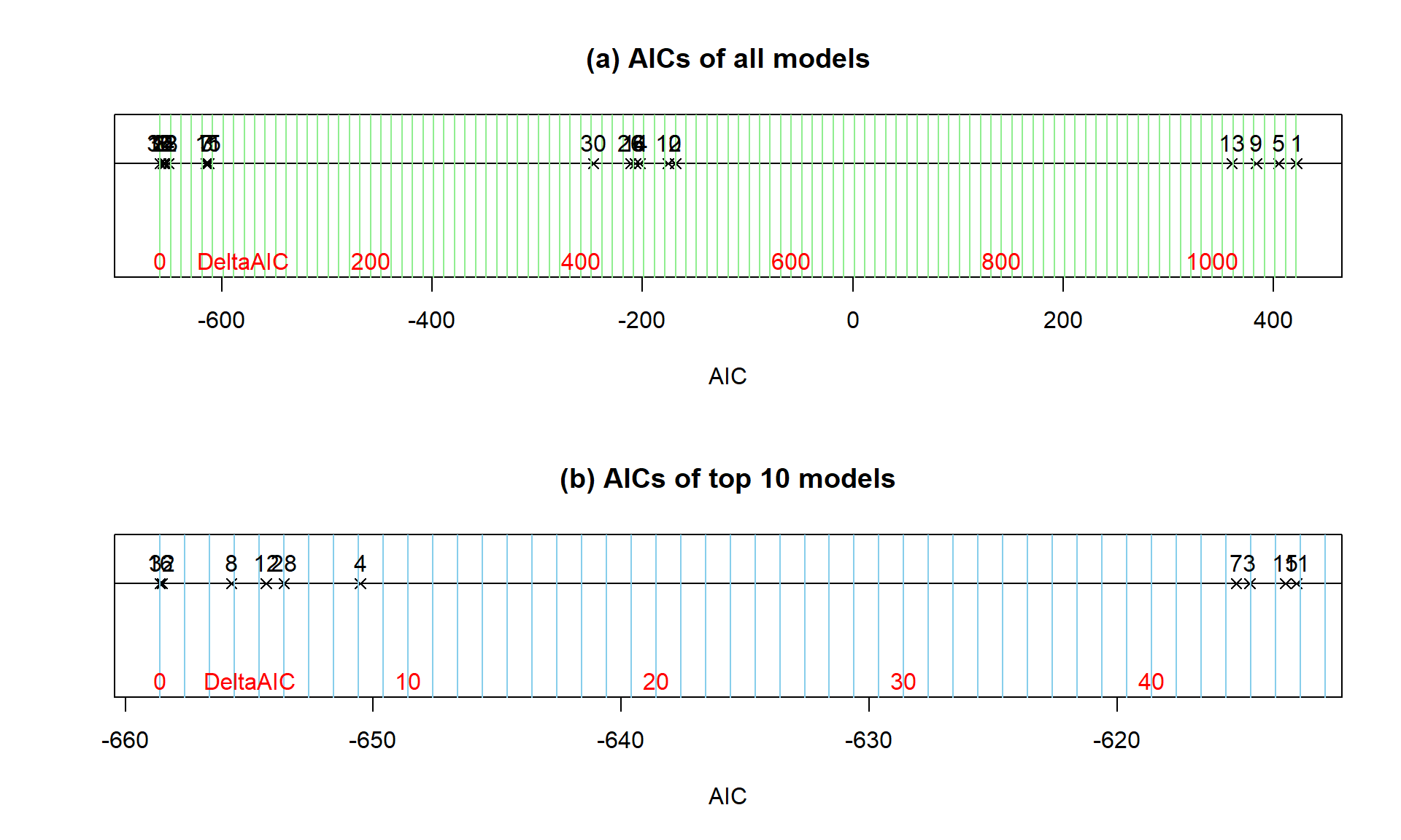— Figure 8.45: Display of AIC results on a number line with models indicated by their number in the `dredge` output. In more complex models, the `dredge` model numbers are just labels and not a meaningful numeration of the models being considered (there are 20 models considered here but labels go up to 32). Panel (a) presents results for all the models and panel (b) focuses just on the top 10 models so some differences in those models can be explored. Note that the spacing of the vertical grid lines in panel (a) are 10 AIC units and in (b) they are 1 AIC unit apart.

The dredge results also provides the opportunity to compare the model selection results from the adjusted R² compared to the AIC. The AIC favors the model without an interaction between age and smoking whereas the adjusted R² favors the most complicated model considered here that included an age and smoking interaction. The AIC provides units that are more interpretable than adjusted R² even though the scale for the AIC is a bit mysterious as distances from the unknown true model with possibly negative distances.

The top AIC model (and possibly the other similar models) can then be explored in more detail. You should not then focus on hypothesis testing in this model. Hypothesis testing so permeates the use of statistics that even after using AICs many researchers are pressured to report p-values for model components. Some of this could be confusion caused when people first learned these statistical methods because when we teach you statistics we show you how to use various methods, one after another, and forget to mention that you should not use every method we taught you in every analysis. Confidence intervals and term-plots are useful for describing the different model components and making inferences for the estimated sizes of differences in the population. These results should not be used for deciding if terms are “significant” when the models (and their components) have already been selected using measures like the AIC or adjusted R². But you can discuss the estimated model components to go with how you arrived at having them in the model.

In this situation, the top model is estimated to be

\[\log(\widehat{\text{FEV}})_i = -1.94 + 0.043\cdot\text{Height}_i+ 0.0234\cdot\text{Age}_i -0.046I_{\text{Smoker},i}+0.0293I_{\text{Male},i}\]

based on the estimated coefficients provided below. Using these results and the term-plots (Figure 8.46) we see that in this model there are positive slopes for Age and Height on log-FEV, a negative coefficient for smoking (Smoker), and a positive coefficient for sex (Males). There is some multicollinearity impacting the estimates for height and age based on having VIFs near 3 but these are not extreme issues. We could go further with interpretations such as for the age term: For a 1 year increase in age, we estimate, on average, a 0.0234 log-liter increase in FEV, after controlling for the height, smoking status, and sex of the children. We can even interpret this on the original scale since this was a log(y) response model using the same techniques as in Section 7.6. If we exponentiate the slope coefficient of the quantitative variable, \(\exp(0.0234) = 1.0237\). This provides the interpretation on the original FEV scale, for a 1 year increase in age, we estimate a 2.4% increase in the median FEV, after controlling for the height, smoking status, and sex of the children. The only difference from Section 7.6 when working with a log(y) model now is that we have to note that the model used to generate the slope coefficient had other components and so this estimate is after adjusting for them.

fm1R$coefficients

## (Intercept)      height         age smokeSmoker     sexMale 
## -1.94399818  0.04279579  0.02338721 -0.04606754  0.02931936

vif(fm1R)

##   height      age    smoke      sex 
## 2.829728 3.019010 1.209564 1.060228

confint(fm1R)

##                    2.5 %       97.5 %
## (Intercept) -2.098414941 -1.789581413
## height       0.039498923  0.046092655
## age          0.016812109  0.029962319
## smokeSmoker -0.087127344 -0.005007728
## sexMale      0.006308481  0.052330236

plot(allEffects(fm1R), grid = T)

Figure 8.46: Term-plots for the top AIC model for log(FEV) that includes height, age, smoking status, and sex in the model.

Like any statistical method, the AIC works better with larger sample sizes and when assumptions are not clearly violated. It also will detect important variables in models more easily when the effects of the predictor variables are strong. Along with the AIC results, it is good to report the coefficients for your top estimated model(s), confidence intervals for the coefficients and/or term-plots, and R². This provides a useful summary of the reasons for selecting the model(s), information on the importance of the terms within the model, and a measure of the variability explained by the model. The R² is not used to select the model, but after selection can be a nice summary of model quality. For fm1R , the \(R^2 = 0.8106\) suggesting that the selected model explains 81% of the variation in log-FEV values.

The AICs are a preferred modeling strategy in some fields such as Ecology. As with this and many other methods discussed in this book, it is sometimes as easy to find journal articles with mistakes in using statistical methods as it is to find papers doing it correctly. After completing this material, you have the potential to have the knowledge and experience of two statistics classes and now are better trained than some researchers that frequently use these methods. This set of tools can be easily mis-applied. Try to make sure that you are thinking carefully through your problem before jumping to the statistical results. Make a graph first, think carefully about your study design and variables collected and what your models of interest might be, what assumptions might be violated based on the data collection story, and then start fitting models. Then check your assumptions and only proceed on with any inference if the conditions are not clearly violated. The AIC provides an alternative method for selecting among different potential models and they do not need to be nested (a requirement of hypothesis testing methods used to sequentially simplify models). The automated consideration of all possible models in the dredge function should not be considered in all situations but can be useful in a preliminary model exploration study where no clear knowledge exists about useful models to consider. Where some knowledge exists of possible models of interest a priori, fit those models and use the AIC function to get AICs to compare. Reporting the summary of AIC results beyond just reporting the top model(s) that were selected for focused exploration provides the evidence to support that selection – not p-values!