8.5: General recommendations for MLR interpretations and VIFs

There are some important issues to remember¹⁴² when interpreting regression models that can result in common mistakes.

• Don’t claim to “hold everything constant” for a single individual:

  Mathematically this is a correct interpretation of the MLR model but it is rarely the case that we could have this occur in real applications. Is it possible to increase the Elevation while holding the Max.Temp constant? We discussed making term-plots doing exactly this – holding the other variables constant at their means. If we interpret each slope coefficient in an MLR conditionally then we can craft interpretations such as: For locations that have a Max.Temp of, say, \(45^\circ F\) and Min.Temp of, say, \(30^\circ F\), a 1 foot increase in Elevation tends to be associated with a 0.0268 inch increase in Snow Depth on average. This does not try to imply that we can actually make that sort of change but that given those other variables, the change for that variable is a certain magnitude.

• Unless you are analyzing the results of a designed experiment (where the levels of the explanatory variable(s) were randomly assigned) you cannot state that a change in that \(x\) causes a change in \(y\), especially for a given individual. The multicollinearity in predictors makes it especially difficult to put too much emphasis on a single slope coefficient because it may be corrupted/modified by the other variables being in the model. In observational studies, there are also all the potential lurking variables that we did not measure or even confounding variables that we did measure but can’t disentangle from the variable used in a particular model. While we do have a complicated mathematical model relating various \(x\text{'s}\) to the response, do not lose that fundamental focus on causal vs non-causal inferences based on the design of the study.
• It is harder to know if you are doing extrapolation in MLR since you could be in a region of the \(x\text{'s}\) that no observations were obtained. Suppose we want to predict the Snow Depth for an Elevation of 6000 and Max.Temp of 30. Is this extrapolation based on Figure 8.16? In other words, can you find any observations “nearby” in the plot of the two variables together? What about an Elevation of 6000 and a Max.Temp of 40? The first prediction is in a different proximity to observations than the second one… In situations with more than two explanatory variables it becomes even more challenging to know whether you are doing extrapolation and the problem grows as the number of dimensions to search increases… In fact, in complicated MLR models we typically do not know whether there are observations “nearby” if we are doing predictions for unobserved combinations of our predictors. Note that Figure 8.16 also reinforces our potential collinearity problem between Elevation and Max.Temp with higher elevations being strongly associated with lower temperatures.

  

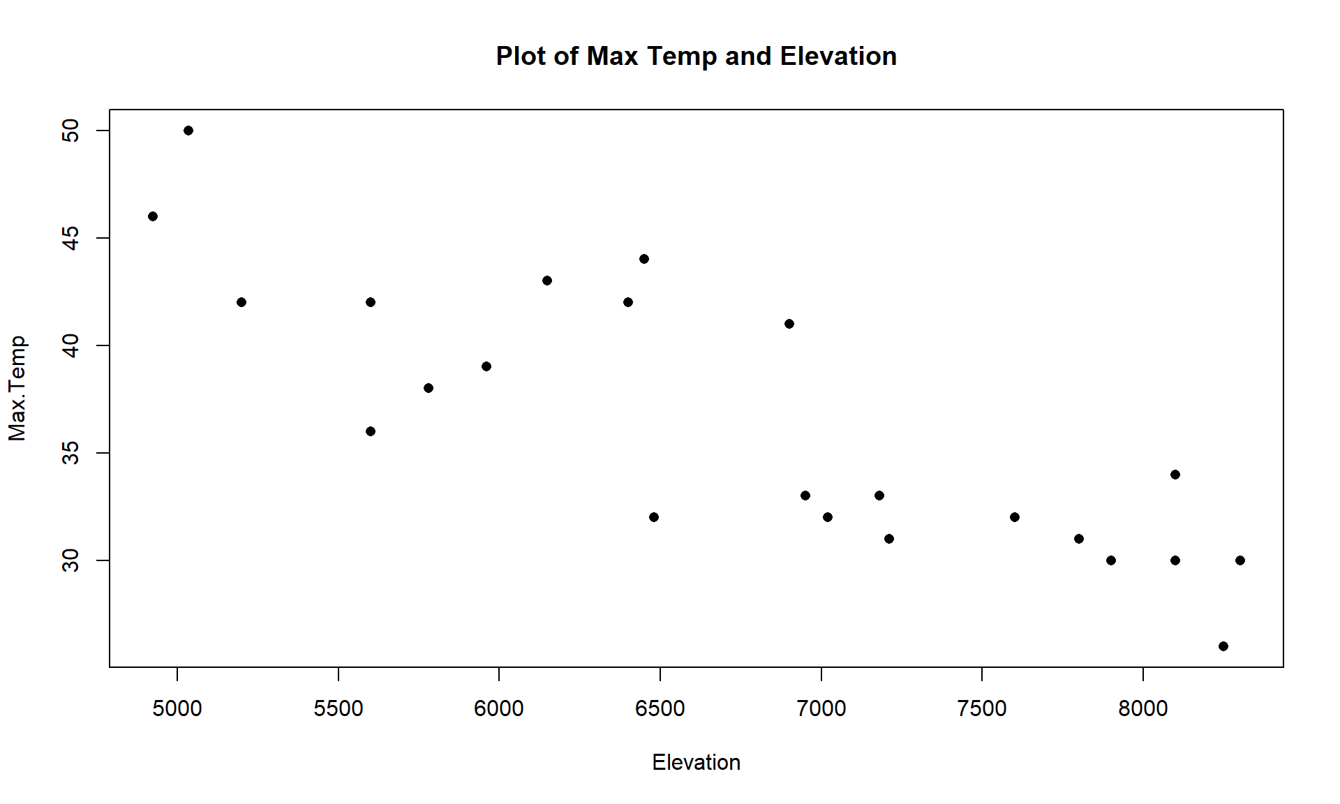
  Figure 8.16: Scatterplot of observed Elevations and Maximum Temperatures for SNOTEL data.

• Adding other variables into the MLR models can cause a switch in the coefficients or change their magnitude or make them go from “important” to “unimportant” without changing the slope too much. This is related to the conditionality of the relationships being estimated in MLR and the potential for sharing of information in the predictors when it is present.
• When explanatory variables are not independent (related) to one another, then including/excluding one variable will have an impact on the other variable. Consider the correlations among the predictors in the SNOTEL data set or visually displayed in Figure 8.17:

  library(corrplot)
  par(mfrow = c(1,1), oma = c(0,0,1,0))
  corrplot.mixed(cor(snotel_s %>% slice(-c(9,22)) %>% select(3:6)), 
                 upper.col = c(1, "orange"), lower.col = c(1, "orange"))
  round(cor(snotel_s %>% slice(-c(9,22)) %>% select(3:6)), 2)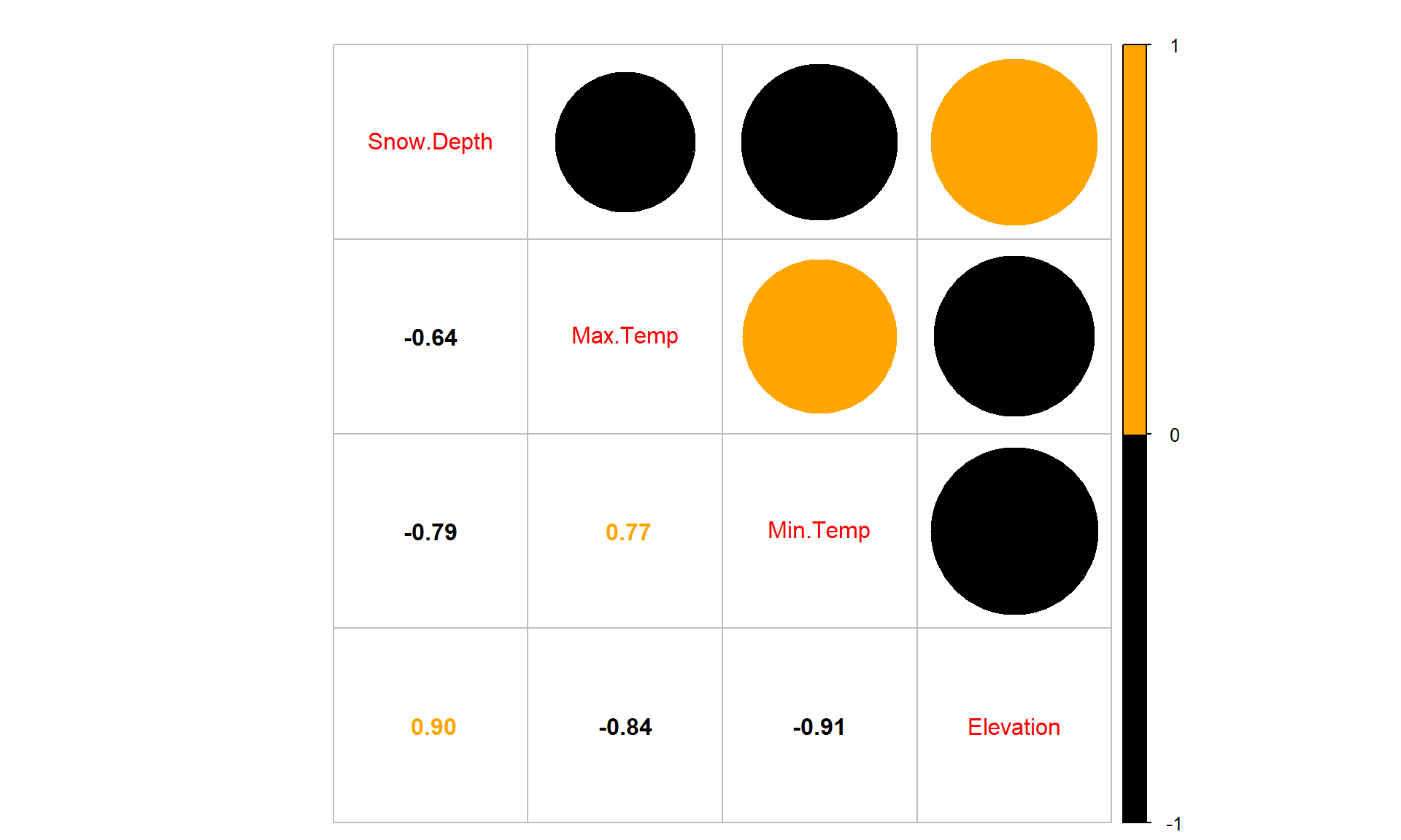

  

  Figure 8.17: Plot of correlation matrix in the snow depth data set with influential points removed

  ##            Snow.Depth Max.Temp Min.Temp Elevation
  ## Snow.Depth       1.00    -0.64    -0.79      0.90
  ## Max.Temp        -0.64     1.00     0.77     -0.84
  ## Min.Temp        -0.79     0.77     1.00     -0.91
  ## Elevation        0.90    -0.84    -0.91      1.00

  The predictors all share at least moderately strong linear relationships. For example, the \(\boldsymbol{r} = -0.91\) between Min.Temp and Elevation suggests that they contain very similar information and that extends to other pairs of variables as well. When variables share information, their addition to models may not improve the performance of the model and actually can make the estimated coefficients unstable, creating uncertainty in the correct coefficients because of the shared information. It seems that Elevation is related to Snow Depth but maybe it is because it has lower Minimum Temperatures? So you might wonder how we can find the “correct” slopes when they are sharing information in the response variable. The short answer is that we can’t. But we do use Least Squares to find coefficient estimates as we did before – except that we have to remember that these estimates are conditional on other variables in the model for our interpretation since they impact one another within the model. It ends up that the uncertainty of pinning those variables down in the presence of shared information leads to larger SEs for all the slopes. And that we can actually measure how much each of the SEs are inflated because of multicollinearity with other variables in the model using what are called Variance Inflation Factors (or VIFs).

VIFs provide a way to assess the multicollinearity in the MLR model that is caused by including specific variables. The amount of information that is shared between a single explanatory variable and the others can be found by regressing that variable on the others and calculating R² for that model. The code for this regression is something like: lm(X1 ~ X2 + X3 + ... + XK), which regresses X1on X2 through XK. The \(1-\boldsymbol{R}^2\) from this regression is the amount of independent information in X1 that is not explained by (or related to) the other variables in the model. The VIF for each variable is defined using this quantity as \(\textbf{VIF}_{\boldsymbol{k}}\boldsymbol{=1/(1-R^2_k)}\) for variable \(k\). If there is no shared information \((\boldsymbol{R}^2 = 0)\), then the VIF will be 1. But if the information is completely shared with other variables \((\boldsymbol{R}^2 = 1)\), then the VIF goes to infinity (1/0). Basically, large VIFs are bad, with the rule of thumb that values over 5 or 10 are considered “large” values indicating high (over 5) or extreme (over 10) multicollinearity in the model for that particular variable, both indicating that slope coefficients are dangerous to interpret in that model. We use this scale to determine if multicollinearity is a definite problem for a variable of interest. But any value of the VIF over 1 indicates some amount of multicollinearity is present. Additionally, the \(\boldsymbol{\sqrt{\textbf{VIF}_k}}\) is also very interesting as it is the number of times larger than the SE for the slope for variable \(k\) is due to collinearity with other variables in the model. The square-root scale is the most useful scale to understand VIFs and allows you to make your own assessment of whether you think the multicollinearity is “important” based on how inflated the SEs are in a particular situation. An example will show how to easily get these results and where the results come from.

In general, the easy way to obtain VIFs is using the vif function from the car package (Fox, Weisberg, and Price (2022b), Fox (2003)). It has the advantage of also providing a reasonable result when we include categorical variables in models (Sections 8.9 and 8.11). We apply the vif function directly to a model of interest and it generates values for each explanatory variable.

library(car)
vif(m6)

## Elevation  Min.Temp  Max.Temp 
##  8.164201  5.995301  3.350914

Not surprisingly, there is an indication of problems with multicollinearity in two of the three variables in the model with the largest issues identified for Elevation and Min.Temp. Both of their VIFs exceed 5 indicating high levels of multicollinearity impacting those terms in the model. On the square-root scale, the VIFs show more interpretation utility.

sqrt(vif(m6))

## Elevation  Min.Temp  Max.Temp 
##  2.857307  2.448530  1.830550

The result for Elevation of 2.86 suggests that the SE for Elevation is 2.86 times larger than it should be because of multicollinearity with other variables in the model. Similarly, the Min.Temp SE is 2.45 times larger and the Max.Temp SE is 1.83 times larger. Even the result for Max.Temp suggests an issue with multicollinearity even though it is below the cut-off for noting high or extreme issues with shared information. All of this generally suggests issues with multicollinearity in the model and that we need to be cautious in interpreting any slope coefficients from this model because they are all being impacted by shared information in the predictor variables to some degree or another.

In order to see how the VIF is calculated for Elevation, we need to regress Elevation on Min.Temp and Max.Temp. Note that this model is only fit to find the percentage of variation in elevation explained by the temperature variables. It ends up being 0.8775 – so a high percentage of Elevation can be explained by the linear model using min and max temperatures.

# VIF calc:
elev1 <- lm(Elevation ~ Min.Temp + Max.Temp, data = snotel_s %>% slice(-c(9,22)))
summary(elev1)

## 
## Call:
## lm(formula = Elevation ~ Min.Temp + Max.Temp, data = snotel_s %>% 
##     slice(-c(9, 22)))
## 
## Residuals:
##      Min       1Q   Median       3Q      Max 
## -1120.05  -142.99    14.45   186.73   624.61 
## 
## Coefficients:
##             Estimate Std. Error t value Pr(>|t|)
## (Intercept) 14593.21     699.77  20.854 4.85e-15
## Min.Temp     -208.82      38.94  -5.363 3.00e-05
## Max.Temp      -56.28      20.90  -2.693    0.014
## 
## Residual standard error: 395.2 on 20 degrees of freedom
## Multiple R-squared:  0.8775, Adjusted R-squared:  0.8653 
## F-statistic: 71.64 on 2 and 20 DF,  p-value: 7.601e-10

Using this result, we can calculate

\[\text{VIF}_{\text{elevation}} = \dfrac{1}{1-R^2_{\text{elevation}}} = \dfrac{1}{1-0.8775} = \dfrac{1}{0.1225} = 8.16\]

1 - 0.8775

## [1] 0.1225

1/0.1225

## [1] 8.163265

Note that when we observe small VIFs (close to 1), that provides us with confidence that multicollinearity is not causing problems under the surface of a particular MLR model and that we can trust that the coefficients will not change dramatically based on whether the other terms in the model are removed. Also note that we can’t use the VIFs to do anything about multicollinearity in the models – it is just a diagnostic to understand the magnitude of the problem.