6.4: Inference for the correlation coefficient

Last updated
Save as PDF

Page ID: 33267

\( \newcommand{\vecs}[1]{\overset { \scriptstyle \rightharpoonup} {\mathbf{#1}} } \) \( \newcommand{\vecd}[1]{\overset{-\!-\!\rightharpoonup}{\vphantom{a}\smash {#1}}} \)\(\newcommand{\id}{\mathrm{id}}\) \( \newcommand{\Span}{\mathrm{span}}\) \( \newcommand{\kernel}{\mathrm{null}\,}\) \( \newcommand{\range}{\mathrm{range}\,}\) \( \newcommand{\RealPart}{\mathrm{Re}}\) \( \newcommand{\ImaginaryPart}{\mathrm{Im}}\) \( \newcommand{\Argument}{\mathrm{Arg}}\) \( \newcommand{\norm}[1]{\| #1 \|}\) \( \newcommand{\inner}[2]{\langle #1, #2 \rangle}\) \( \newcommand{\Span}{\mathrm{span}}\) \(\newcommand{\id}{\mathrm{id}}\) \( \newcommand{\Span}{\mathrm{span}}\) \( \newcommand{\kernel}{\mathrm{null}\,}\) \( \newcommand{\range}{\mathrm{range}\,}\) \( \newcommand{\RealPart}{\mathrm{Re}}\) \( \newcommand{\ImaginaryPart}{\mathrm{Im}}\) \( \newcommand{\Argument}{\mathrm{Arg}}\) \( \newcommand{\norm}[1]{\| #1 \|}\) \( \newcommand{\inner}[2]{\langle #1, #2 \rangle}\) \( \newcommand{\Span}{\mathrm{span}}\)\(\newcommand{\AA}{\unicode[.8,0]{x212B}}\)

We used bootstrapping briefly in Chapter 2 to generate nonparametric confidence intervals based on the middle 95% of the bootstrapped version of the statistic. Remember that bootstrapping involves sampling with replacement from the data set and creates a distribution centered near the statistic from the real data set. This also mimics sampling under the alternative as opposed to sampling under the null as in our permutation approaches. Bootstrapping is particularly useful for making confidence intervals where the distribution of the statistic may not follow a named distribution. This is the case for the correlation coefficient which we will see shortly.

The correlation is an interesting summary but it is also an estimator of a population parameter called \(\rho\) (the symbol rho), which is the population correlation coefficient. When \(\rho = 1\), we have a perfect positive linear relationship in the population; when \(\rho = -1\), there is a perfect negative linear relationship in the population; and when \(\rho = 0\), there is no linear relationship in the population. Therefore, to test if there is a linear relationship between two quantitative variables, we use the null hypothesis \(H_0: \rho = 0\) (tests if the true correlation, \(\rho\), is 0 – no linear relationship). The alternative hypothesis is that there is some (positive or negative) relationship between the variables in the population, \(H_A: \rho \ne 0\). The distribution of the Pearson correlation coefficient can be complicated in some situations, so we will use bootstrapping methods to generate confidence intervals for \(\rho\) based on repeated random samples with replacement from the original data set. If the \(C\%\) confidence interval contains 0, then we would find little to no evidence against the null hypothesis since 0 is in the interval of our likely values for \(\rho\). If the \(C\%\) confidence interval does not contain 0, then we would find strong evidence against the null hypothesis. Along with its use in testing, it is also interesting to be able to generate a confidence interval for \(\rho\) to provide an interval where we are \(C\%\) confident that the true parameter lies.

The beers and BAC example seemed to provide a strong relationship with \(\boldsymbol{r} = 0.89\). As correlations approach -1 or 1, the sampling distribution becomes more and more skewed. This certainly shows up in the bootstrap distribution that the following code produces (Figure 6.10). Remember that bootstrapping utilizes the resample function applied to the data set to create new realizations of the data set by re-sampling with replacement from those observations. The bold vertical line in Figure 6.10 corresponds to the estimated correlation \(\boldsymbol{r} = 0.89\) and the distribution contains a noticeable left skew with a few much smaller \(T^*\text{'s}\) possible in bootstrap samples. The \(C\%\) confidence interval is found based on the middle \(C\%\) of the distribution or by finding the values that put \((100-C)/2\) into each tail of the distribution with the qdata function.

Tobs <- cor(BAC ~ Beers, data = BB); Tobs

## [1] 0.8943381

set.seed(614)
B <- 1000
Tstar <- matrix(NA, nrow = B)
for (b in (1:B)){
  Tstar[b] <- cor(BAC ~ Beers, data = resample(BB))
}
quantiles <- qdata(Tstar, c(0.025, 0.975)) #95% Confidence Interval

quantiles

##      2.5%     97.5% 
## 0.7633606 0.9541518

tibble(Tstar) %>% ggplot(aes(x = Tstar)) +
  geom_histogram(aes(y = ..ncount..), bins = 15, col = 1, fill = "skyblue", center = 0) +
  geom_density(aes(y = ..scaled..)) +
  theme_bw() +
  labs(y = "Density") +
  geom_vline(xintercept = quantiles, col = "blue", lwd = 2, lty = 3) +
  geom_vline(xintercept = Tobs, col = "red", lwd = 2) +
  stat_bin(aes(y = ..ncount.., label = ..count..), bins = 15,
           geom = "text", vjust = -0.75)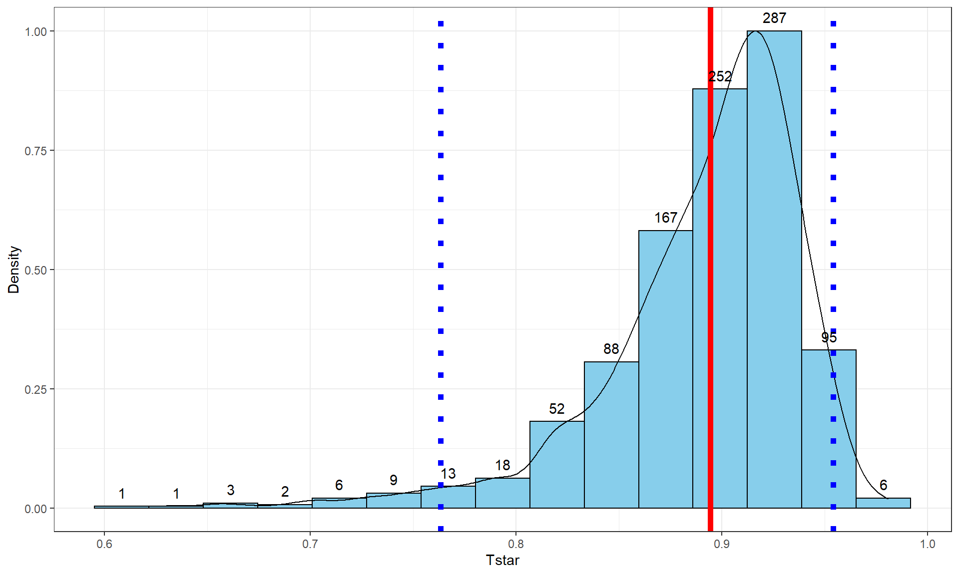

Figure 6.10: Histogram and density curve of the bootstrap distribution of the correlation coefficient with bold vertical line for observed correlation and dashed lines for bounds for the 95% bootstrap confidence interval.

These results tell us that the bootstrap 95% CI is from 0.76 to 0.95 – we are 95% confident that the true correlation between Beers and BAC in all OSU students like those that volunteered for this study is between 0.76 and 0.95. Note that there are no units on the correlation coefficient or in this interpretation of it.

We can also use this confidence interval to test for a linear relationship between these variables.

\(\boldsymbol{H_0:\rho = 0:}\) There is no linear relationship between Beers and BAC in the population.
\(\boldsymbol{H_A: \rho \ne 0:}\) There is a linear relationship between Beers and BAC in the population.

The 95% confidence level corresponds to a 5% significance level test and if the 95% CI does not contain 0, you know that the p-value would be less than 0.05 and if it does contain 0 that the p-value would be more than 0.05. The 95% CI is from 0.76 to 0.95, which does not contain 0, so we find strong evidence¹¹⁵ against the null hypothesis and conclude that there is a linear relationship between Beers and BAC in OSU students. We’ll revisit this example using the upcoming regression tools to explore the potential for more specific conclusions about this relationship. Note that for these inferences to be accurate, we need to be able to trust that the sample correlation is reasonable for characterizing the relationship between these variables along with the assumptions we will discuss below.

In this situation with randomly assigned levels of \(x\) and strong evidence against the null hypothesis of no relationship, we can further conclude that changing beer consumption causes changes in the BAC. This is a much stronger conclusion than we can typically make based on correlation coefficients. Correlations and scatterplots are enticing for infusing causal interpretations in non-causal situations. Statistics teachers often repeat the mantra that correlation is not causation and that generally applies – except when there is randomization involved in the study. It is rarer for researchers either to assign, or even to be able to assign, levels of quantitative variables so correlations should be viewed as non-causal unless the details of the study suggest otherwise.