6.5: Are tree diameters related to tree heights?

In a study at the Upper Flat Creek study area in the University of Idaho Experimental Forest, a random sample of \(n = 336\) trees was selected from the forest, with measurements recorded on Douglas Fir, Grand Fir, Western Red Cedar, and Western Larch trees. The data set called ufc is available from the spuRs package (Jones et al. 2018) and contains dbh.cm (tree diameter at 1.37 m from the ground, measured in cm) and height.m (tree height in meters). The relationship displayed in Figure 6.11 is positive, moderately strong with some curvature and increasing variability as the diameter increases. There do not appear to be groups in the data set but since this contains four different types of trees, we would want to revisit this plot by type of tree. To assist in the linearity assessment, we also add the geom_smooth to the plot with an option of method = "lm", which provides a straight line to best describe the relationship (more on that line in the coming sections and chapters). The bands around the line are based on the 95% confidence intervals we can generate for any x-value and relate to pinning down the true mean value of the y-variable at that value of the x-variable – but only apply if the linear relationship is a good description of the relationship between the variables (which it is not here!).

library(spuRs) #install.packages("spuRs")
data(ufc)
ufc <- as_tibble(ufc)

ufc %>% ggplot(mapping = aes(x = dbh.cm, y = height.m)) +
  geom_point() +
  geom_smooth(method = "lm") +
  theme_bw()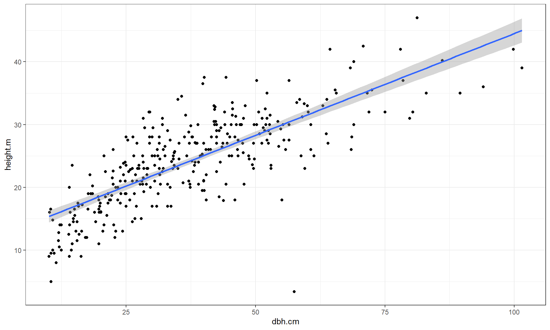 

Figure 6.11: Scatterplot of tree heights (m) vs tree diameters (cm) with estimated straight line relationship (blue line) and 95% confidence interval (grey band).

Of particular interest is an observation with a diameter around 58 cm and a height of less than 5 m. Observing a tree with a diameter around 60 cm is not unusual in the data set, but none of the other trees with this diameter had heights under 15 m. It ends up that the likely outlier is in observation number 168 and because it is so unusual it likely corresponds to either a damaged tree or a recording error.

ufc %>% slice(168)

## # A tibble: 1 × 5
##    plot  tree species dbh.cm height.m
##   <int> <int> <fct>    <dbl>    <dbl>
## 1    67     6 WL        57.5      3.4

With the outlier in the data set, the correlation is 0.77 and without it, the correlation increases to 0.79. The removal does not create a big change because the data set is relatively large and the diameter value is close to the mean of the \(x\text{'s}\)¹¹⁶ but it has some impact on the strength of the correlation.

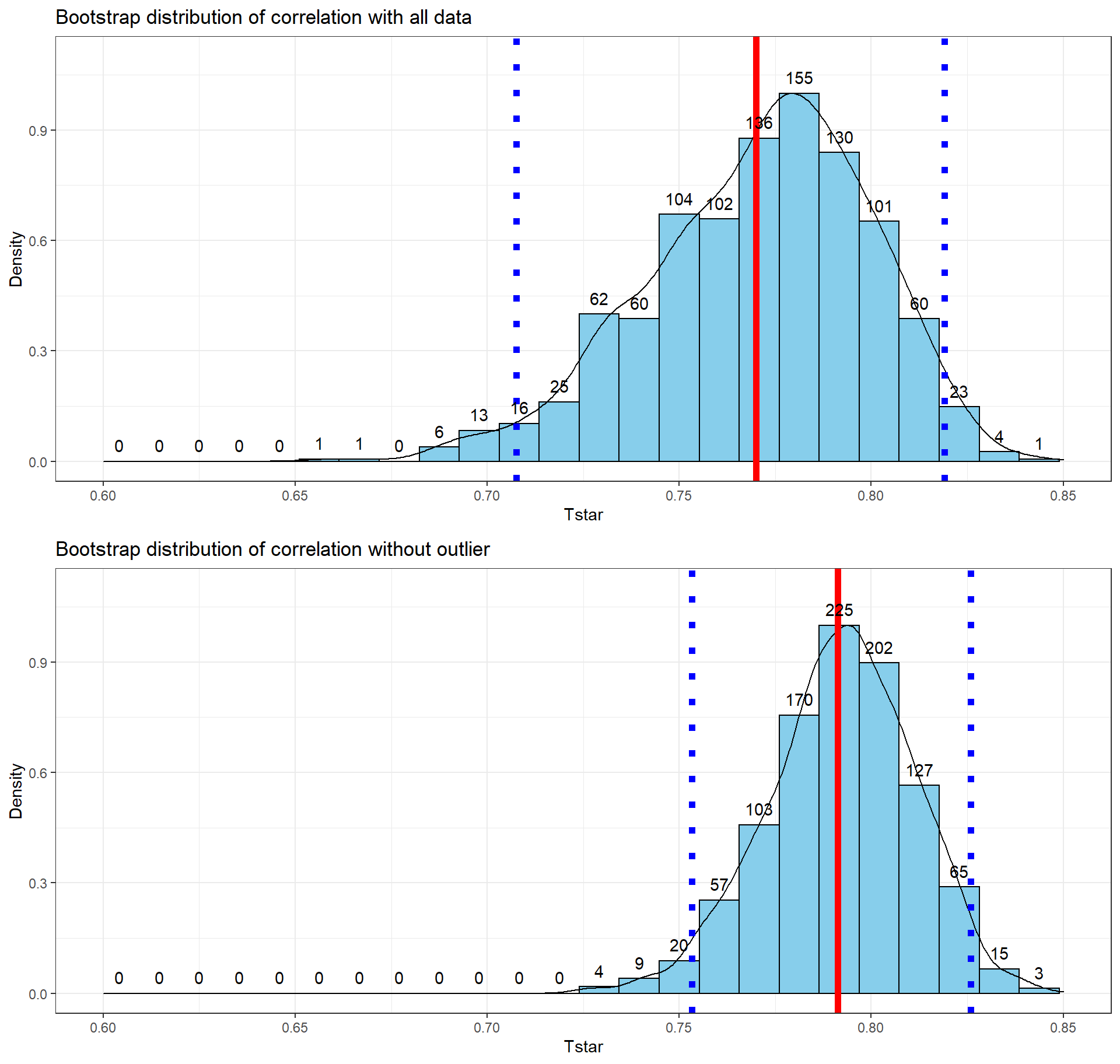
cor(dbh.cm ~ height.m, data = ufc)

## [1] 0.7699552

cor(dbh.cm ~ height.m, data = ufc %>% slice(-168))

## [1] 0.7912053

With the outlier included, the bootstrap 95% confidence interval goes from 0.702 to 0.820 – we are 95% confident that the true correlation between diameter and height in the population of trees is between 0.708 and 0.819. When the outlier is dropped from the data set, the 95% bootstrap CI is 0.753 to 0.826, which shifts the lower endpoint of the interval up, reducing the width of the interval from 0.111 to 0.073 (Figure 6.12). In other words, the uncertainty regarding the value of the population correlation coefficient is reduced. The reason to remove the observation is that it is unusual based on the observed pattern, which implies an error in data collection or sampling from a population other than the one used for the other observations and, if the removal is justified, it helps us refine our inferences for the population parameter. But measuring the linear relationship in these data where there is a clear curve violates one of our assumptions of using these methods – we’ll see some other ways of detecting this issue in Section 6.10 and we’ll try to “fix” this example using transformations in Chapter 7.

Tobs <- cor(dbh.cm ~ height.m, data = ufc); Tobs

## [1] 0.7699552

set.seed(208)
B <- 1000
Tstar <- matrix(NA, nrow = B)
for (b in (1:B)){
  Tstar[b] <- cor(dbh.cm ~ height.m, data = resample(ufc))
}
quantiles <- qdata(Tstar, c(.025, .975)) #95% Confidence Interval
quantiles

##      2.5%     97.5% 
## 0.7075771 0.8190283

p1 <- tibble(Tstar) %>%  ggplot(aes(x = Tstar)) +
  geom_histogram(aes(y = ..ncount..), bins = 25, col = 1, fill = "skyblue", center = 0) +
  geom_density(aes(y = ..scaled..)) +
  theme_bw() +
  labs(y = "Density", title = "Bootstrap distribution of correlation with all data") +
  geom_vline(xintercept = quantiles, col = "blue", lwd = 2, lty = 3) +
  geom_vline(xintercept = Tobs, col = "red", lwd = 2) +
  stat_bin(aes(y = ..ncount.., label = ..count..), bins = 25,
           geom = "text", vjust = -0.75) +
  xlim(0.6, 0.85) +
  ylim(0, 1.1)

Tobs <- cor(dbh.cm ~ height.m, data = ufc %>% slice(-168)); Tobs

## [1] 0.7912053

Tstar <- matrix(NA, nrow = B)
for (b in (1:B)){
  Tstar[b] <- cor(dbh.cm ~ height.m, data = resample(ufc %>% slice(-168)))
}
quantiles <- qdata(Tstar, c(.025, .975)) #95% Confidence Interval
quantiles

##      2.5%     97.5% 
## 0.7532338 0.8259416

p2 <- tibble(Tstar) %>%  ggplot(aes(x = Tstar)) +
  geom_histogram(aes(y = ..ncount..), bins = 25, col = 1, fill = "skyblue", center = 0) + 
  geom_density(aes(y = ..scaled..)) +
  theme_bw() +
  labs(y = "Density", title = "Bootstrap distribution of correlation without outlier") +
  geom_vline(xintercept = quantiles, col = "blue", lwd = 2, lty = 3) +
  geom_vline(xintercept = Tobs, col = "red", lwd = 2) +
  stat_bin(aes(y = ..ncount.., label = ..count..), bins = 25,
           geom = "text", vjust = -0.75) +
  xlim(0.6, 0.85) +
  ylim(0, 1.1)

grid.arrange(p1, p2, ncol = 1)

Figure 6.12: Bootstrap distributions of the correlation coefficient for the full data set (top) and without potential outlier included (bottom) with observed correlation (bold line) and bounds for the 95% confidence interval (dashed lines). Notice the change in spread of the bootstrap distributions as well as the different centers.