1.1: Overview of methods

This book is designed primarily for use in a second semester statistics course although it can also be useful for researchers needing a quick review or ideas for using R for the methods discussed in the text. As a text primarily designed for a second statistics course, it presumes that you have had an introductory statistics course. There are now many different varieties of introductory statistics from traditional, formula-based courses (called “consensus” curriculum courses) to more modern, computational-intensive courses that use randomization ideas to try to enhance learning of basic statistical methods. We are not going to presume that you have had a particular “flavor” of introductory statistics or that you had your introductory statistics out of a particular text, just that you have had a course that tried to introduce you to the basic terminology and ideas underpinning statistical reasoning. We would expect that you are familiar with the logic (or sometimes illogic) of hypothesis testing including null and alternative hypothesis and confidence interval construction and interpretation and that you have seen all of this in a couple of basic situations. We start with a review of these ideas in one and two group situations with a quantitative response, something that you should have seen before.

This text covers a wide array of statistical tools that are connected through situation, methods used, or both. As we explore various techniques, look for the identifying characteristics of each method – what type of research questions are being addressed (relationships or group differences, for example) and what type of variables are being analyzed (quantitative or categorical). Quantitative variables are made up of numerical measurements that have meaningful units attached to them. Categorical variables take on values that are categories or labels. Additionally, you will need to carefully identify the response and explanatory variables, where the study and variable characteristics should suggest which variables should be used as the explanatory variables that may explain variation in the response variable. Because this is an intermediate statistics course, we will start to handle more complex situations (many explanatory variables) and will provide some tools for graphical explorations to complement the more sophisticated statistical models required to handle these situations.

1.1 Overview of methods

After you are introduced to basic statistical ideas, a wide array of statistical methods become available. The methods explored here focus on assessing (estimating and testing for) relationships between variables, sometimes when controlling for or modifying relationships based on levels of another variable – which is where statistics gets interesting and really useful. Early statistical analyses (approximately 100 years ago) were focused on describing a single variable. Your introductory statistics course should have heavily explored methods for summarizing and doing inference in situations with one group or where you were comparing results for two groups of observations. Now, we get to consider more complicated situations – culminating in a set of tools for working with multiple explanatory variables, some of which might be categorical and related to having different groups of subjects that are being compared. Throughout the methods we will cover, it will be important to retain a focus on how the appropriate statistical analysis depends on the research question and data collection process as well as the types of variables measured.

Figure 1.1 frames the topics we will discuss. Taking a broad view of the methods we will consider, there are basically two scenarios – one when the response is quantitative and one when the response is categorical. Examples of quantitative responses we will see later involve passing distance of cars for a bicycle rider (in centimeters (cm)) and body fat (percentage). Examples of categorical variables include improvement (none, some, or marked) in a clinical trial related to arthritis symptoms or whether a student has turned in copied work (never, done this on an exam or paper, or both). There are going to be some more nuanced aspects to all these analyses as the complexity of both sides of Figure 1.1 suggest, but note that near the bottom, each tree converges on a single procedure, using a linear model for a quantitative response variable or using a Chi-square test for a categorical response. After selecting the appropriate procedure and completing the necessary technical steps to get results for a given data set, the final step involves assessing the scope of inference and types of conclusions that are appropriate based on the design of the study.

Figure 1.1: Flow chart of methods.

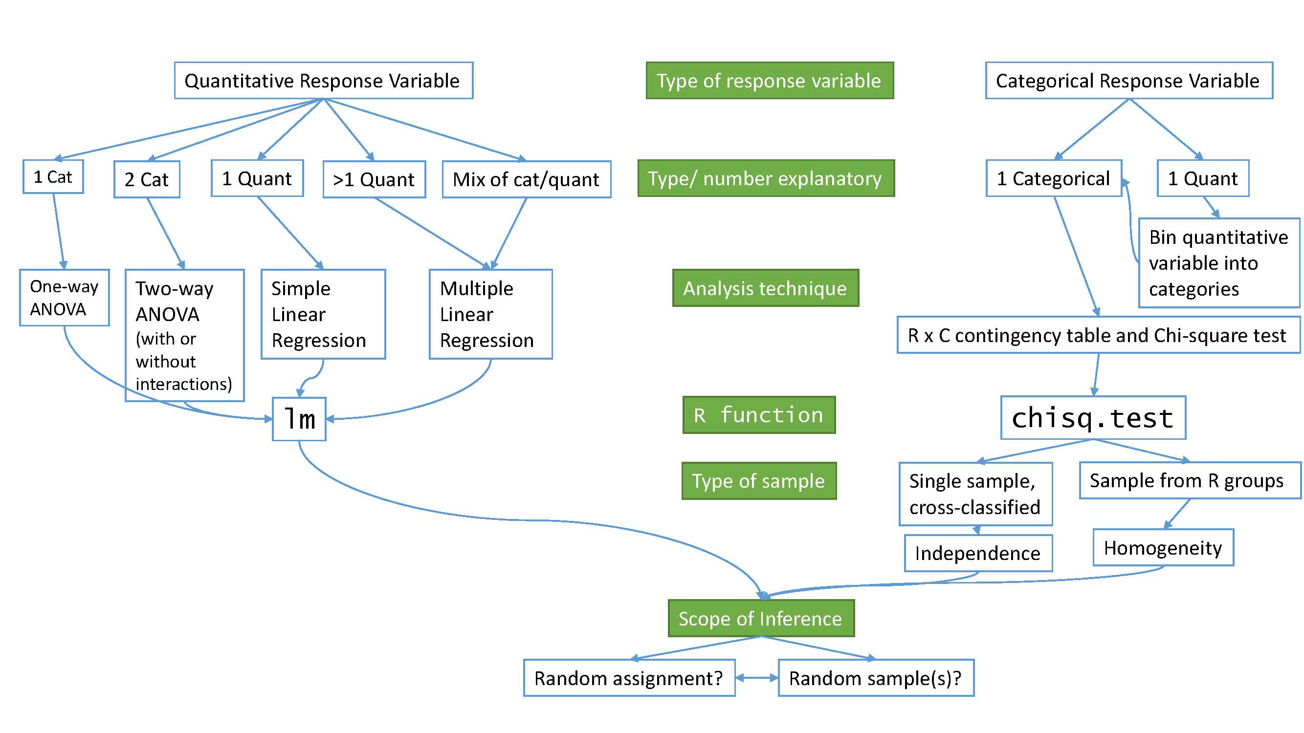
We will be spending most of the semester working on methods for quantitative response variables (the left side of Figure 1.1 is covered in Chapters 2, 3, 4, 6, 7, and 8), stepping over to handle the situation with a categorical response variable in Chapter 5 (right side of Figure 1.1). Chapter 9 contains case studies illustrating all the methods discussed previously, providing a final opportunity to explore additional examples that illustrate how finding a path through Figure 1.1 can lead to the appropriate analysis.

The first topics (Chapters 1, and 2) will be more familiar as we start with single and two group situations with a quantitative response. In your previous statistics course, you should have seen methods for estimating and quantifying uncertainty for the mean of a single group and for differences in the means of two groups. Once we have briefly reviewed these methods and introduced the statistical software that we will use throughout the course, we will consider the first new statistical material in Chapter 3. It involves the situation with a quantitative response variable where there are more than 2 groups to compare – this is what we call the One-Way ANOVA situation. It generalizes the 2-independent sample hypothesis test to handle situations where more than 2 groups are being studied. When we learn this method, we will begin discussing model assumptions and methods for assessing those assumptions that will be present in every analysis involving a quantitative response. The Two-Way ANOVA (Chapter 3) considers situations with two categorical explanatory variables and a quantitative response. To make this somewhat concrete, suppose we are interested in assessing differences in, say, the yield of wheat from a field based on the amount of fertilizer applied (none, low, or high) and variety of wheat (two types). Here, yield is a quantitative response variable that might be measured in bushels per acre and there are two categorical explanatory variables, fertilizer, with three levels, and variety, with two levels. In this material, we introduce the idea of an interaction between the two explanatory variables: the relationship between one categorical variable and the mean of the response changes depending on the levels of the other categorical variable. For example, extra fertilizer might enhance the growth of one variety and hinder the growth of another so we would say that fertilizer has different impacts based on the level of variety. Given this interaction may or may not actually be present, we will consider two versions of the model in Two-Way ANOVAs, what are called the additive (no interaction) and the interaction models.

Following the methods for two categorical variables and a quantitative response, we explore a method for analyzing data where the response is categorical, called the Chi-square test in Chapter 5. This most closely matches the One-Way ANOVA situation with a single categorical explanatory variable, except now the response variable is categorical. For example, we will assess whether taking a drug (vs taking a placebo¹) has an effect² on the type of improvement the subjects demonstrate. There are two different scenarios for study design that impact the analysis technique and hypotheses tested in Chapter 5. If the explanatory variable reflects the group that subjects were obtained from, either through randomization of the treatment level to the subjects or by taking samples from separate populations, this is called a Chi-square Homogeneity Test. It is also possible to obtain a single sample from a population and then obtain information on the levels of the explanatory variable for each subject. We will analyze these results using what is called a Chi-square Independence Test. They both use the same test statistic but we use slightly different graphics and are testing different hypotheses in these two related situations. Figure 1.1 also shows that if we had a quantitative explanatory variable and a categorical response that we would need to “bin” or create categories of responses from the quantitative variable to use the Chi-square testing methods.

If the predictor and response variables are both quantitative, we start with scatterplots, correlation, and simple linear regression models (Chapters 6 and 7) – things you should have seen, at least to some degree, previously. The biggest differences here will be the depth of exploration of diagnostics and inferences for this model and discussions of transformations of variables. If there is more than one explanatory variable, then we say that we are doing multiple linear regression (Chapter 8) – the “multiple” part of the name reflects that there will be more than one explanatory variable. We use the same name if we have a mix of categorical and quantitative predictor variables but there are some new issues in setting up the models and interpreting the coefficients that we need to consider. In the situation with one categorical predictor and one quantitative predictor, we revisit the idea of an interaction. It allows us to consider situations where the estimated relationship between a quantitative predictor and the mean response varies among different levels of the categorical variable. In Chapter 9, connections among all the methods used for quantitative responses are discussed, showing that they are all just linear models . We also show how the methods discussed can be applied to a suite of new problems with a set of case studies and how that relates to further extensions of the methods.

By the end of Chapter 9 you should be able to identify, perform using the statistical software R (R Core Team 2022), and interpret the results from each of these methods. There is a lot to learn, but many of the tools for using R and interpreting results of the analyses accumulate and repeat throughout the textbook. If you work hard to understand the initial methods, it will help you when the methods get more complicated. You will likely feel like you are just starting to learn how to use R at the end of the semester and for learning a new language that is actually an accomplishment. We will just be taking you on the first steps of a potentially long journey and it is up to you to decide how much further you want to go with learning the software.

All the methods you will learn require you to carefully consider how the data were collected, how that pertains to the population of interest, and how that impacts the inferences that can be made. The scope of inference from the bottom of Figure 1.1 is our shorthand term for remembering to think about two aspects of the study – random assignment and random sampling. In a given situation, you need to use the description of the study to decide if the explanatory variable was randomly assigned to study units (this allows for causal inferences if differences are detected) or not (so no causal statements are possible). As an example, think about two studies, one where students are randomly assigned to either get tutoring with their statistics course or not and another where the students are asked at the end of the semester whether they sought out tutoring or not. Suppose we compare the final grades in the course for the two groups (tutoring/not) and find a big difference. In the first study with random assignment, we can say the tutoring caused the differences we observed. In the second, we could only say that the tutoring was associated with differences but because students self-selected the group they ended up in, we can’t say that the tutoring caused the differences. The other aspect of scope of inference concerns random sampling: If the data were obtained using a random sampling mechanism, then our inferences can be safely extended to the population that the sample was taken from. However, if we have a non-random sample, our inference can only apply to the sample collected. In the previous example, the difference would be studying a random sample of students from the population of, say, Introductory Statistics students at a university versus studying a sample of students that volunteered for the research project, maybe for extra credit in the class. We could still randomly assign them to tutoring/not but the non-random sample would only lead to conclusions about those students that volunteered. The most powerful scope of inference is when there are randomly assigned levels of explanatory variables with a random sample from a population – conclusions would be about causal impacts that would happen in the population.

By the end of this material, you should have some basic R skills and abilities to create basic ANOVA and regression models, as well as to handle Chi-square testing situations. Together, this should prepare you for future statistics courses or for other situations where you are expected to be able to identify an appropriate analysis, do the calculations and required graphics using the data set, and then effectively communicate interpretations for the methods discussed here.