5.2: Nested Treatment Design

When setting up a multi-factor study, sometimes it is not possible to cross the factor levels. In other words, because of the logistics of the situation, we may not be able to have each level of treatment be combined with each level of another treatment.

Here is an example:

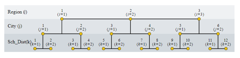
A research team interested in the lifestyle of high school students conducted a study to compare the activity levels of high school students across the 3 geographic regions in the United States, Northeast (NE), Midwest (MW), and the West (W). The study also included the comparison of activity levels among cities within each region. Two school districts were chosen from two major cities from each of these 3 regions and the response variable, the average number of exercise hours per week for high school students for each school district was recorded.

A diagram to illustrate the treatment design can be set up as follows. Here, the subscript \(i\) identifies the regions, and the subscript \(j\) indicates the cities:

Factor A (Region) \(i\)		Factor B (City) \(j\)		Average
		1	2
NE		30	18
		35	20
	Average	\(\bar{Y}_{11.}=32.5\)	\(\bar{Y}_{12.}=19\)	\(\bar{Y}_{1..}=25.75\)
MW		10	20
		9	22
	Average	\(\bar{Y}_{21.}=9.5\)	\(\bar{Y}_{22.}=21\)	\(\bar{Y}_{2..}=15.25\)
W		18	4
		19	6
	Average	\(\bar{Y}_{31.}=18.5\)	\(\bar{Y}_{32.}=5\)	\(\bar{Y}_{3..}=9.5\)
			Average	\(\bar{Y}_{...}=16.83\)

The table above shows the data obtained: the grand mean, the marginal means which are the treatment level means, and finally, the cell means. The cell means are the averages of the two school district mean activity levels for each combination of Region and City.

This example drives home the point that the levels of the second factor (City) cannot practically be crossed with the levels of the first factor (Region) as cities are specific or unique to regions. Note that the cities are identified as 1 or 2 within each region. But it is important to note that city 1 in the Northeast is not the same as city 1 in the Midwest. The concept of nesting does come in useful to describe this type of situation and the use of parentheses is appropriate to clearly indicate the nesting of factors. To indicate that the City is nested within the factor Region, the notation: City(Region) will be used. Here, City is the nested factor and Region is the nesting factor.

Figure \(\PageIndex{1}\): Diagram of the levels of treatment design.

We can partition the deviations as before into the following components: \[\underbrace{Y_{ijk} - \bar{Y}_{...}}_{\text{Total deviation}} = \underbrace{\bar{Y}_{i..} - \bar{Y}_{...}}_{\text{A main effect}} + \underbrace{\bar{Y}_{ij.} - \bar{Y}_{i..}}_{\text{Specific B effect when A at the } i^{th} \text{ level}} + \underbrace{Y_{ijk} - \bar{Y}_{ij.}}_{\text{Residual}}\]

Source	d.f.
Region	\((a- 1) = 2\)
City (Region)	\(a(b-1) = 3\)
Error	\(ab(n-1) = 6\)
Total	\(N - 1 = 11\)

The statistical model follows as: \[Y_{ijk} = \mu + \alpha_{i} + \beta_{j(i)} + \epsilon_{ijk}\] \[\begin{aligned} \text{where: } & \mu \text{ is a constant} \\ &\alpha_{i} \text{ are constants subject to the restriction } \sum \alpha_{i} = 0 \\ &\beta_{j(i)} \text{ are constants subject to the restriction } \sum \beta_{j(i)} = 0 \text{ for all } i \\ &\epsilon_{ijk} \text{ are independent } N \left(0, \sigma^2\right) \\ &i = 1, \ldots, a; \ j = 1, \ldots, b; \ k = 1, \ldots, n \end{aligned}

We will want to test the following Null Hypotheses:

For Factor A

\[H_{0}: \ \mu_{\text{Northeast}} = \mu_{\text{Midwest}} = \mu_{\text{West}} \text{ vs. } H_{A}: \ \text{Not all equal}\]

For Factor B

When stating the Null Hypothesis for Factor B, the nested effect, alternative notation has to be used.

Up to this point, we have been stating Null Hypotheses in terms of the means (e.g. \(H_{0}:\ \mu_{1} = \mu_{2} = \ldots = \mu_{k}\)), but we can alternatively state a Null Hypothesis in terms of the parameters for that treatment in the model. For example, for the nesting factor A, we could also state the Null Hypothesis as \[H_{0}: \ \alpha_{\text{Northeast}} = \alpha_{\text{Midwest}} = \alpha_{\text{West}} = 0 \text{ or } H_{0}: \ \text{all } \alpha_{i} = 0\]

For the nested factor B, the Null Hypothesis should differentiate between the nesting and the nested factors, because we are evaluating the nested factor within the levels of the nesting factor.

So for the nested factor (City, nested within Region), we have the Null Hypothesis. \[H_{0}: \ \text{all } \beta_{j(i)} = 0 \text{ vs. } H_{A}: \ \text{not all } \beta_{j(i)} = 0 \text{ for } j=1, 2,\]

The \(F\)-tests can then proceed as usual using the ANOVA results. The first two columns of the ANOVA table should be as follows on the next page.

Note

1. There is no interaction between a nested factor and its nesting factor.
2. The nested factors always have to be accompanied by their nested factor. This means that the effect B does not exist and B(A) represents the effect of B within the factor A
3. df of B(A) = df of B + df of A*B (This is simply a mathematically correct identity and may not be of much practical use, as effects B(A) and A*B cannot coexist)
4. The residual effect of any ANOVA model is a nested effect - the replicate effect nested within the factor level combinations. Recall that the replicates are considered homogeneous and so any variability among them serves to estimate the model error.