5.1.2: Two-Factor Factorial - Greenhouse Example (Minitab)

Last updated
Save as PDF

Page ID: 33635

\( \newcommand{\vecs}[1]{\overset { \scriptstyle \rightharpoonup} {\mathbf{#1}} } \) \( \newcommand{\vecd}[1]{\overset{-\!-\!\rightharpoonup}{\vphantom{a}\smash {#1}}} \)\(\newcommand{\id}{\mathrm{id}}\) \( \newcommand{\Span}{\mathrm{span}}\) \( \newcommand{\kernel}{\mathrm{null}\,}\) \( \newcommand{\range}{\mathrm{range}\,}\) \( \newcommand{\RealPart}{\mathrm{Re}}\) \( \newcommand{\ImaginaryPart}{\mathrm{Im}}\) \( \newcommand{\Argument}{\mathrm{Arg}}\) \( \newcommand{\norm}[1]{\| #1 \|}\) \( \newcommand{\inner}[2]{\langle #1, #2 \rangle}\) \( \newcommand{\Span}{\mathrm{span}}\) \(\newcommand{\id}{\mathrm{id}}\) \( \newcommand{\Span}{\mathrm{span}}\) \( \newcommand{\kernel}{\mathrm{null}\,}\) \( \newcommand{\range}{\mathrm{range}\,}\) \( \newcommand{\RealPart}{\mathrm{Re}}\) \( \newcommand{\ImaginaryPart}{\mathrm{Im}}\) \( \newcommand{\Argument}{\mathrm{Arg}}\) \( \newcommand{\norm}[1]{\| #1 \|}\) \( \newcommand{\inner}[2]{\langle #1, #2 \rangle}\) \( \newcommand{\Span}{\mathrm{span}}\)\(\newcommand{\AA}{\unicode[.8,0]{x212B}}\)

For Minitab, we also need to convert the data to a stacked format (Lesson 4 2 way Stacked Dataset). Once we do this, we will need to use a different set of commands to generate the ANOVA. We use...

Stat > ANOVA > General Linear Model > Fit General Linear Model

and get the following dialog box:

General Linear Model pop-up window with "resp" in the Responses window, and "fert species" in the Factors window. — Figure \(\PageIndex{1}\): General Linear Model pop-up window.

Click on Model…, hold down the shift key and highlight both factors. Then click on the Add box to add the interaction to the model.

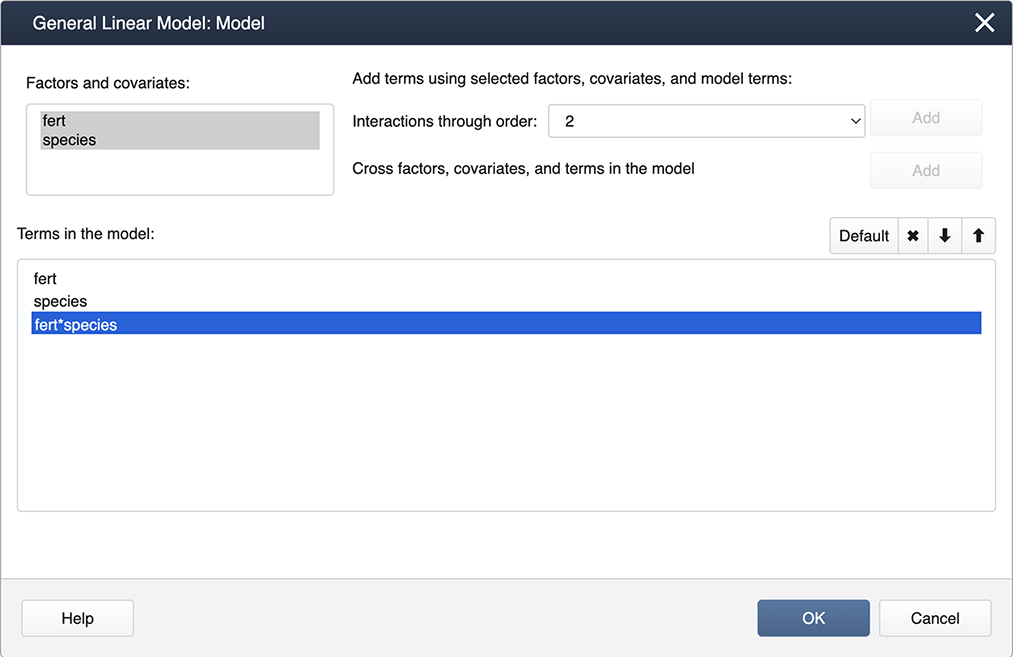
General Linear Model: Model pop-up window with both "fert" and "species" selected in the Factors and covariates window, the value "2" selected in the interactions through order dropdown, and "fert*species" selected in the Terms in the model window. — Figure \(\PageIndex{2}\): General Linear Model: Model pop-up window.

These commands will produce the ANOVA results below which are similar to the output generated by SAS (shown in the previous section).

Analysis of Variance

Source	DF	Adj SS	Adj MS	F-value	P-value
fert	3	745.44	248.479	73.10	0.000
species	1	236.74	236.741	69.65	0.000
fert*species	3	50.58	16.861	4.96	0.005
Error	40	135.97	3.399
Total	47	1168.73

Following the ANOVA run, you can generate the mean comparisons by

Stat > ANOVA > General Linear Model > Comparisons

Then specify the fert*species interaction term for the comparisons by checking the box.

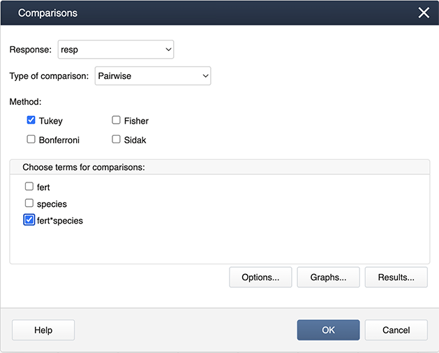
Comparisons pop-up window with "resp" selected in the Response dropdown, "Pairwise" selected in the Type of comparison dropdown, "Tukey" selected as the method and "fert*species" selected as the terms for comparison. — Figure \(\PageIndex{3}\): Comparisons pop-up window.

Then choose Graphs to get the following dialog box, where "Interval plot for difference of means" should be checked.

Comparisons: Graphs pop-up window, with "Interval plot for differences of means" checked. — Figure \(\PageIndex{4}\): Comparisons: Graphs pop-up window.

The outputs are shown below.

Grouping Information Using the Tukey Method and 95% Confidence

fert	species	N	Mean	Grouping
f3	SppB	6	37.0667	A
f1	SppB	6	31.6167	B
f2	SppB	6	30.0500	B
f3	SppA	6	29.2000	B C
f1	SppA	6	28.6000	B C
f2	SppA	6	25.8667	C D
control	SppB	6	23.7000	D E
control	SppA	6	21.0000	E

Means that do not share a letter are significantly different.

Minitab Tukey Simultaneous 95% confidence intervals graph of differences of means for resp. — Figure \(\PageIndex{5}\): Tukey simultaneous 95% confidence intervals.