5.1: Factorial or Crossed Treatment Designs

In multi-factor experiments, combinations of factor levels are applied to experimental units. The single-factor greenhouse experiment discussed in previous lessons can be extended to a multi-factor study by including plant species as an additional factor along with fertilizer type. This addition of another factor may prove to be useful, as one fertilizer type may be most effective on one specific plant species! In other words, the optimal height growth is perhaps attainable by a unique combination of fertilizer type and plant species. A treatment design that provides the opportunity to determine this best combination is a factorial design, where responses are observed at each level of a given factor combined with each level of all other factors. In this setting, factors are said to be crossed.

A factorial design with \(t\) factors is identified using the \(l_{1} l_{2} \ldots l_{t}\) notation, where \(l_{i}\) is the number of levels of factor \(i\) \((i=1,2, \ldots,t)\). For example, a factorial design with 2 factors A and B, where A has 4 levels and B has 3 levels, will have the \(4 \times 3\) notation.

One complete replication of a factorial design with \(t\) factors requires \((l_{1} \times l_{2} \times \ldots \times l_{t})\) experimental units, and this quantity is called the replicate size. If \(r\) is the number of complete replicates, then \(N\), the total number of observations, equals \(r \times (l_{1} \times l_{2} \times \ldots \times l_{t})\).

It is easy to see that with the addition of more and more crossed factors, the replicate size will increase rapidly and design modifications have to be made to make the experiment more manageable.

In a factorial experiment, as combinations of different factor levels play an important role, it is important to differentiate between the lone (or main) effects of a factor on the response and the combined effects of a group of factors on the response.

The main effect of factor A is the effect of A on the response ignoring the effect of all other factors. The main effect of a given factor is equivalent to the factor effect associated with the single-factor experiment using only that particular factor.

The combined effect of a specific combination of \(l\) different factors is called the interaction effect (more details later). The interaction effect of most interest is the two-way interaction effect and is denoted by the product of the two letters assigned to the two factors. For example, the two-way interaction effects of a factorial design with 3 factors A, B, C are denoted AB, AC, and BC. Likewise, the three-way interaction effect of these 3 factors is denoted by ABC.

Let us now examine how the degrees of freedom (\(df\)) values of a single-factor ANOVA can be extended to the ANOVA of a two-factor factorial design. Note that the interaction effects are additional terms that need to be included in a multi-factor ANOVA, but the ANOVA rules studied in Chapter 2 for single-factor situations still apply for the main effect of each factor. If the two factors of the design are denoted by A and B with \(a\) and \(b\) as their number of levels respectively, then the \(df\) values of the two main effects are \((a-1)\) and \((b-1)\). The \(df\) value for the two-way interaction effect is \((a-1)(b-1)\), the product of \(df\) values for A and B. The ANOVA table below gives the layout of the df values for a \(2 \times 2\) factorial design with 5 complete replications. Note that in this experiment, \(r\) equals 5, and \(N\) is equal to 20.

Source	d.f.
Factor A	\((a - 1) = 1\)
Factor B	\((b - 1) = 1\)
Factor A × Factor B	\((a - 1)(b - 1) = 1\)
Error	\(19 - 3 = 16\)
Total	\(N-1=(nab)-1=19\)

If in the single-factor model of \[Y_{ij} = \mu + \tau_{i} + \epsilon_{ij}\] \(\tau_{i}\) is effectively replaced with \(\alpha_{i} + \beta_{i} + (\alpha \beta)_{ij}\), then the resulting equation shown below will represent the model equation of a two-factor factorial design.

\[Y_{ijk} = \mu + \alpha_{i} + \beta_{j} + (\alpha \beta)_{ij} + \epsilon_{ijk}\] where \(\alpha_{i}\) is the main effect of factor A, \(\beta_{j}\) is the main effect of factor B, and \((\alpha \beta)_{ij}\) is the interaction effect \((i=1,2,\ldots,a, \ j=1,2,\ldots,b, \ k=1,2,\ldots,r)\).

This reflects the following partitioning of treatment deviations from the grand mean: \[\underbrace{ \bar{Y}_{ij.} - \bar{Y}_{...} }_{\begin{array}{c} \text{Deviation of estimated treatment mean} \\ \text{around overall mean} \end{array}} = \underbrace{ \bar{Y}_{i..} - \bar{Y}_{...} }_{A \text{ main effect}} + \underbrace{ \bar{Y}_{.j.}-\bar{Y}_{...} }_{B \text{ main effect}} + \underbrace{ \bar{Y}_{ij.} - \bar{Y}_{i..} - \bar{Y}_{.j.} + \bar{Y}_{...} }_{AB \text{ interaction effect}} \]

The main effects for Factor A and Factor B are straightforward to interpret, but what is an interaction? Delving more, an interaction can be defined as the failure of the response to one factor to be the same at different levels of another factor. Notice that \((\alpha \beta)_{ij}\), the interaction term in the model, is multiplicative, and as a result may have a large and important impact on the response variable. Interactions go by different names in various fields. In medicine, for example, physicians most times ask what medication you are on before prescribing a new medication. They do this out of a concern for interaction effects of either interference (a canceling effect) or synergism (a compounding effect).

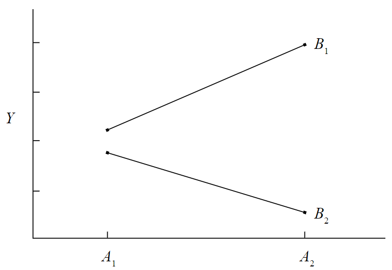
Graphically, in a two-factor factorial with each factor having 2 levels, the interaction can be represented by two non-parallel lines connecting means (adapted from Zar, H. Biostatistical Analysis, 5th Ed., 1999). It is because the interaction reflects the failure of the difference in response between the two different levels of one factor to be the same, for both levels of the other factor. So, if there is no interaction, then this difference in response will be the same, which will graphically result in two parallel lines. In the interaction plots below, parallel lines are a consistent feature in all settings with no interaction. In plots depicting interaction, the lines do cross (or would cross if the lines kept going).

Graph 1 In graph 1 there is no effect of Factor A, a small effect of Factor B (and if there were no effect of Factor B the two lines would coincide), and no interaction between Factor A and Factor B.	Graph 2 Graph 2 shows a large effect of Factor A, small effect of Factor B, and no interaction.
Graph 3 Graph 3 shows no effect of Factor A, larger effect of Factor B, and no interaction.	Graph 4 In graph 4 there is a large effect of Factor A, a large effect of Factor B , and no interaction.
Graph 5 In graph 5 there is no effect of Factor A and no effect of Factor B, but an interaction between A and B.	Graph 6 In graph 6 there is a large effect of Factor A and no effect of Factor B, with a slight interaction between A and B.
Graph 7 In graph 7 there is no effect of Factor A and a large effect of Factor B, with a very large interaction.	Graph 8 In graph 8 there is a small effect of Factor A and a large effect of Factor B, with a large interaction.

In the presence of multiple factors with their interactions, multiple hypotheses can be tested and for a two-factor factorial design. They are:

Main Effect of Factor A:

\[\begin{array}{l} H_{0}: \ \alpha_{1} = \alpha_{2} = \ldots = \alpha_{a} = 0 \\ H_{A}: \ \text{not all } \alpha_{i} \text{ are equal to 0} \end{array}\]

Main Effect of Factor B:

\[\begin{array}{l} H_{0}: \ \beta_{1} = \beta_{2} = \ldots = \beta_{b} = 0 \\ H_{A}: \ \text{not all } \beta_{j} \text{ are equal to 0} \end{array}\]

A × B Interaction:

\[\begin{array}{c} H_{0} \ \text{there is no interaction} \\ H_{A}: \ \text{an interaction exists} \end{array}\]

When testing these hypotheses, it is important to test for the significance of the interaction effect first. If the interaction is significant, the main effects are of no consequence; rather, the differences among different factor level combinations should be looked into. The greenhouse example, extended to include a second (crossed) factor, will illustrate the steps.