3.7: One-Way ANOVA Greenhouse Example in R

R Instructions: Code for the Greenhouse Data

• Load the greenhouse data.
• Calculate the overall mean, standard deviation, and standard error.
• Calculate the mean, standard deviation, and standard error for each group.
• Produce a boxplot to plot the differences in heights for each fertilizer.
• Produce a "means plot" (interval plot) to view the differences in heights for each fertilizer.
• Obtain the ANOVA table.
• Obtain Tukey’s multiple comparisons CIs and difference in means plot.
• Produce diagnostic (residuals) plots.
• Power analysis.

setwd("~/path-to-folder/")
greenhouse_data<-read.table("greenhouse_data.txt",header=T)

Note that greenhouse data are in separate columns.

attach(greenhouse_data)
my_data<-stack(greenhouse_data)

With this command, we put our data in a stacked format (the first column has the response variable (values) and the second column has the treatment levels (ind).

To calculate the overall mean, standard deviation, and standard error we can use the following commands:

overall_mean<-mean(my_data$values) #26.16667
overall_sd<-sd(my_data$values) #3.685892
overall_standard_error<-overall_sd/sqrt(length(my_data$values)) #0.7523795

To calculate the group means we can use the following command:

group_means<-aggregate(my_data[, 1],list(my_data$ind),mean)
#  group_means
#  Group.1        x
# 1 Control 21.00000
# 2      F1 28.60000
# 3      F2 25.86667
# 4      F3 29.20000

To calculate the group standard deviations and standard errors we can use the following commands:

group_sd<-aggregate(my_data[, 1],list(my_data$ind),sd)
# group_sd  Group.1        x
# 1 Control 1.000000
# 2      F1 2.437212
# 3      F2 1.899123
# 4      F3 1.288410

group_standard_error<-group_sd$x/sqrt(length(my_data$ind)/4)
# group_standard_error
# 0.4082483 0.9949874 0.7753136 0.5259911

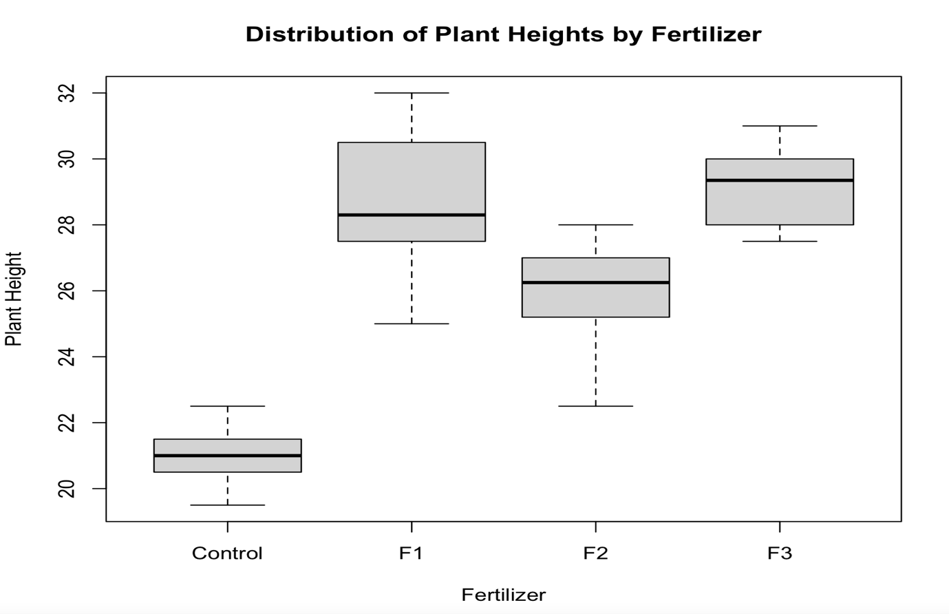
To produce the Boxplot we can use the following commands:

library("ggpubr")       
boxplot(values~ind,data=my_data,
xlab="Fertilizer",ylab="Plant Height",
main="Distribution of Plant Heights by Fertilizer",
frame=TRUE)

Figure \(\PageIndex{1}\): Box plot for distribution of plant heights by fertilizer.

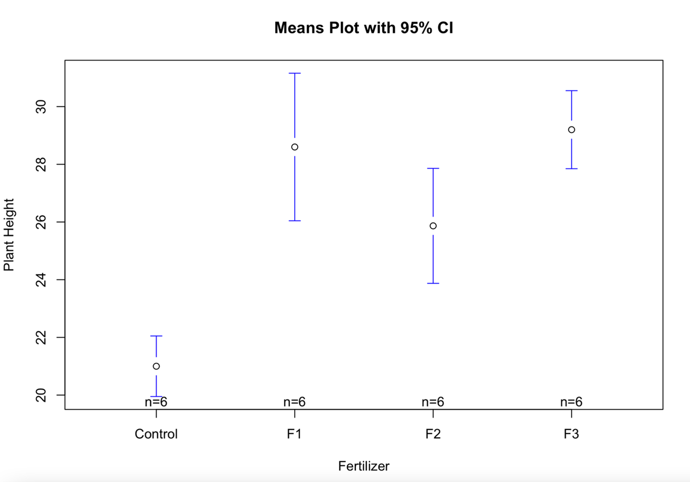
To produce the means plot (interval plot) we can use the following commands:

library("gplots")
plotmeans(values~ind,data=my_data,connect=FALSE,
xlab="Fertilizer",ylab="Plant Height",
main="Means Plot with 95% CI")

Figure \(\PageIndex{2}\): Means plot with 95% confidence interval.

To obtain the ANOVA table we can use the following commands:

anova<-aov(values~ind,my_data)
summary(anova)

The command summary (anova) will give you the following output:

summary(anova)
Df Sum Sq Mean Sq F value   Pr(>F)    
ind          3 251.44   83.81   27.46 2.71e-07 ***
Residuals   20  61.03    3.05                     
---
Signif. codes:  0 ‘***’ 0.001 ‘**’ 0.01 ‘*’ 0.05 ‘.’ 0.1 ‘ ’ 1

We can see the degrees of freedom in the first column, the sum of squares in the second column, the mean sum of squares in the third column, the \(F\)-test statistic in the fourth column, and finally, we can see the \(p\)-value.

Note that the output doesn't give the \(SSTO\). To find it, use the identity \(SSTO=SSR+SSE\). Similarly, for the \(df\) associated with \(SSTO\), add the \(df\) of \(SSR\) and \(SSE\).

For our example, \(SSTO=251.44+61.03=312.47\)

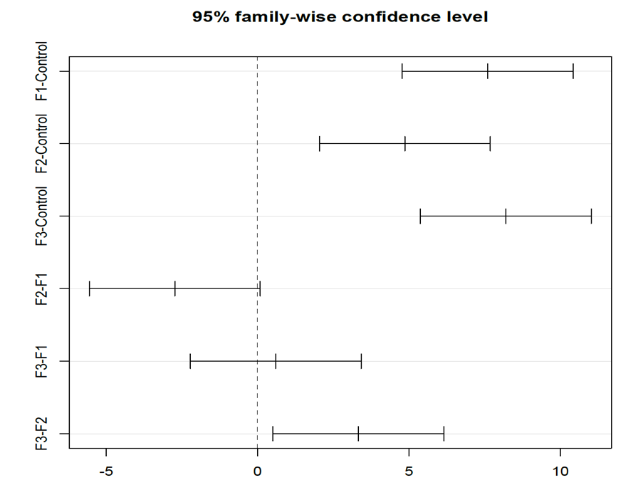
To obtain Tukey multiple comparisons of means with a 95% family-wise confidence level we use the following command:

library(multcomp)
library(multcompView)
tukey_multiple_comparisons<-TukeyHSD(anova,conf.level=0.95)
plot(tukey_multiple_comparisons)
tukey_multiple_comparisons
Tukey multiple comparisons of means
95% family-wise confidence level
Fit: aov(formula = values ~ ind, data = my_data)
$ind
diff        lwr         upr     p adj
F1-Control  7.600000  4.7770648 10.42293521 0.0000016
F2-Control  4.866667  2.0437315  7.68960188 0.0005509
F3-Control  8.200000  5.3770648 11.02293521 0.0000005
F2-F1      -2.733333 -5.5562685  0.08960188 0.0598655
F3-F1       0.600000 -2.2229352  3.42293521 0.9324380
F3-F2       3.333333  0.5103981  6.15626854 0.0171033

Based on this output, the Control group is significantly different from the 3 treatment groups and F3 is significantly different from F2.

Figure \(\PageIndex{3}\): 95% famil-wise confidence level plot.

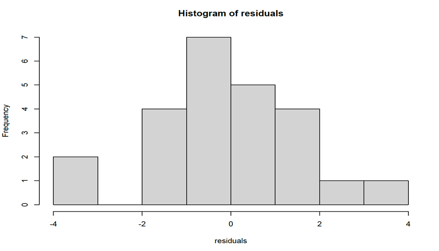
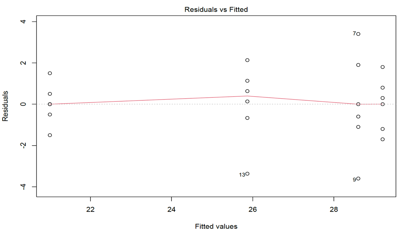
To produce diagnostic (residuals) plots we use the following commands:

#Residuals vs Fits plot
plot(anova,1)

Figure \(\PageIndex{6}\): Residuals vs fitted values plot.

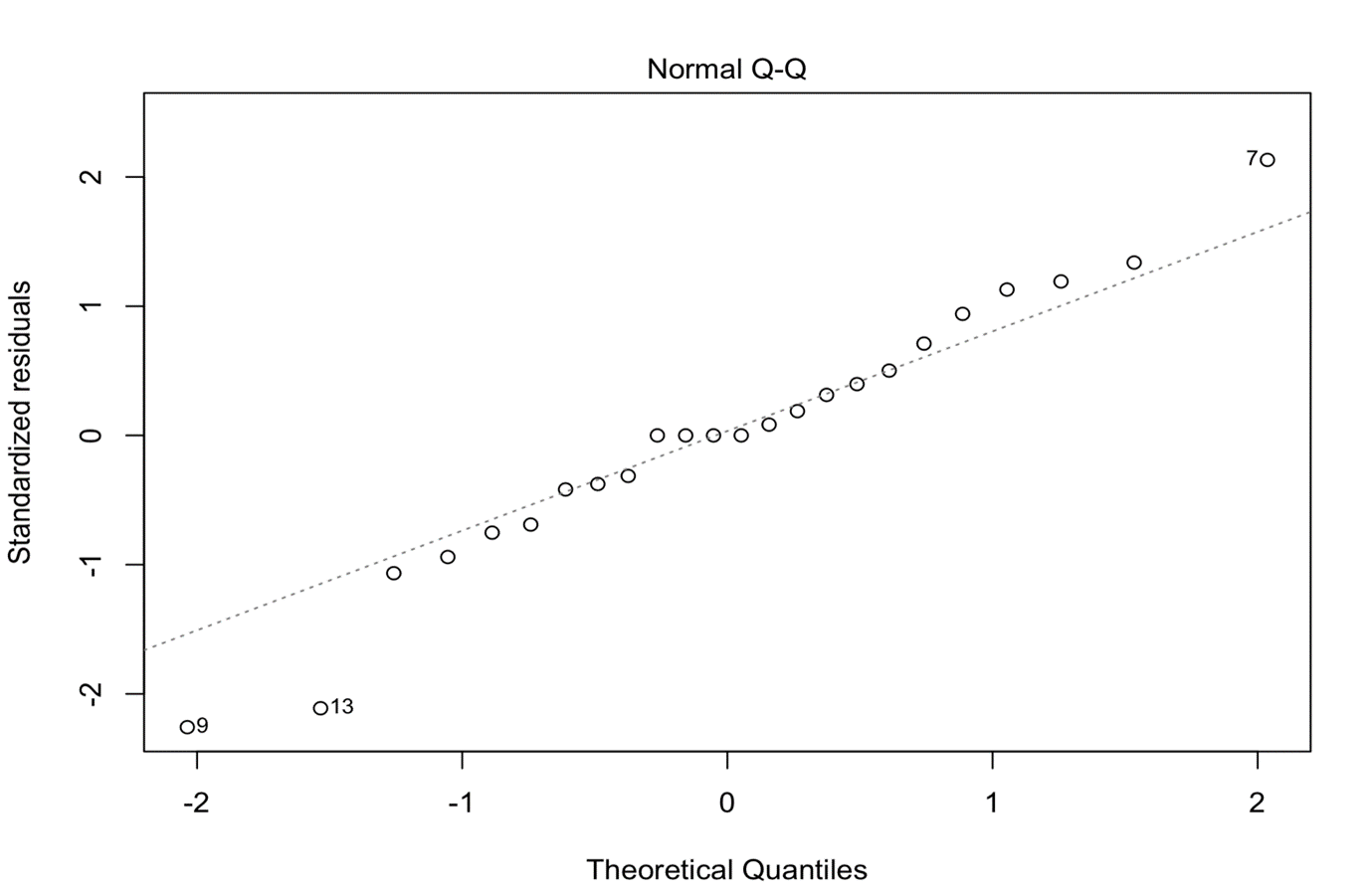
#QQ plot
plot(anova,2)

Figure \(\PageIndex{7}\): Normal Q-Q plot.

#Histogram of residuals
residuals<-anova$res #with this command we get the residuals from ANOVA
hist(residuals)

Figure \(\PageIndex{8}\): Histogram of residuals.