3.8: Power Analysis

After completing a statistical test, conclusions are drawn about the null hypothesis. In cases where the null hypothesis is not rejected, a researcher may still feel that the treatment did have an effect. Let's say that three weight loss treatments are conducted. At the end of the study, the researcher analyzes the data and finds there are no differences among the treatments. The researcher believes that there really are differences. While you might think this is just wishful thinking on the part of the researcher, there MAY be a statistical reason for the lack of significant findings.

At this point, the researcher can run a power analysis. Recall from your introductory text or course that power is the ability to reject the null when the null is really false. The factors that impact power are sample size (larger samples lead to more power), the effect size (treatments that result in larger differences between groups will have differences that are more readily found), the variability of the experiment, and the significance of the type 1 error.

As a note, the most common type of power analysis are those that calculate needed sample sizes for experimental designs. These analyses take advantage of pilot data or previous research. When power analysis is done ahead of time, it is a PROSPECTIVE power analysis. This example is a retrospective power analysis, as it is done after the experiment is completed.

So back to our greenhouse example. Typically we want power to be at 80%. Again, power represents our ability to reject the null when it is false, so a power of 80% means that 80% of the time our test identifies a difference in at least one of the means correctly. The converse of this is that 20% of the time we risk not rejecting the null when we really should be rejecting the null.

Using our greenhouse example, we can run a retrospective power analysis (just a reminder, we typically don't do this unless we have some reason to suspect the power of our test was very low).

This is one analysis where Minitab is much easier and still just as accurate as SAS, so we will use Minitab to illustrate this simple power analysis in detail and follow up the analysis with SAS.

Power Analysis Techniques

Using SAS

Steps in SAS

Let us now consider running the power analysis in SAS. In our greenhouse example with 4 treatments (control, F1, F2, and F3), the estimated means were \(21, 28.6, 25.877, 29.2\) respectively. Using ANOVA, the estimated standard deviation of errors was 1.747 (which is obtained by \(\sqrt{MSE}=\sqrt{3.0517}\). There are 6 replicates for each treatment. Using these values, we could employ SAS POWER procedure to compute the power of our study retrospectively.

proc power;
onewayanova alpha=.05 test=overall
groupmeans=(21 28.6 25.87, 29.2)
npergroup=6 stddev=1.747
power=.;
run;

Fixed Scenario Elements
Method	Exact
Alpha	0.05
Group Means	21 28.6 25.87 29.2
Standard Deviation	1.747
Sample Size per Group	6

Computed Power
Power
>.999

As with MINITAB, we see that the retrospective power analysis for our greenhouse example yields a power of 1. If we re-do the analysis ignoring the CONTROL treatment group, then we only have 3 treatment groups: F1, F2, and F3. The ANOVA with only these three treatments yields an MSE of \(3.735556\). Therefore the estimated standard deviation of errors would be \(1.933\). We will have a power of 0.731 in this modified scenario, as shown in the below output.

Fixed Scenario Elements
Method	Exact
Alpha	0.05
Group Means	28.6 25.87 29.2
Standard Deviation	1.933
Sample Size per Group	6

Computed Power
Power
0.731

Suppose, we ask the question of how many replicates we would need to obtain at least 80% power to detect a difference in the means of our greenhouse example with the same group means but with different variability in data (i.e. standard deviations should be different). We can use SAS POWER to answer this question.

Figure \(\PageIndex{a1}\): Plot for overall \(F\)-test.

We can see that with a standard deviation of 1.747, if we have only 2 replicates in each of the four treatments we can detect the differences in greenhouse example means with more than 80% power. However, as the data get noisier (i.e. as standard deviation increases) we need more replicates to achieve 80% power in the same example.

Using Minitab

Steps in Minitab

In Minitab select STAT > Power and Sample Size > One-Way ANOVA

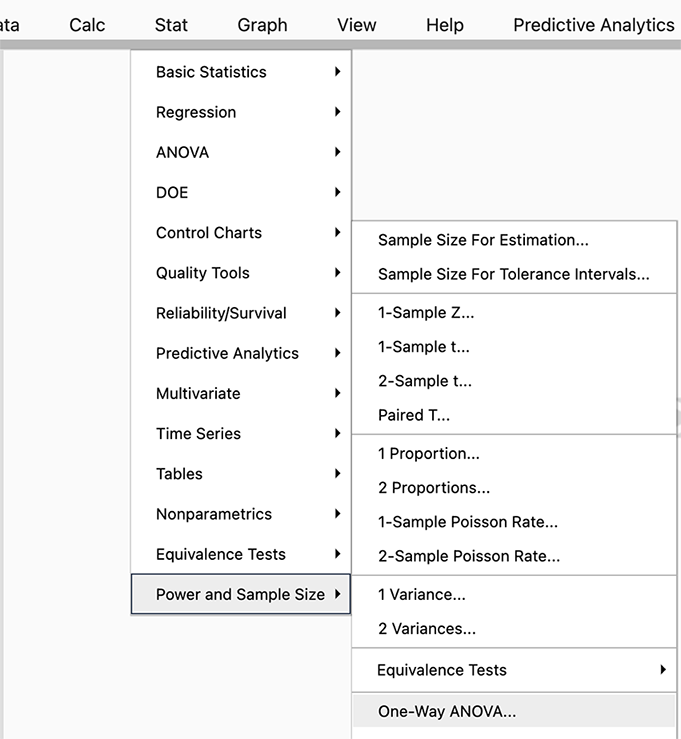
Figure \(\PageIndex{b1}\): Selecting the One-Way ANOVA tab in Minitab.

Since we have a one-way ANOVA we select this test (you can see there are power analyses for many different tests, and SAS will allow even more complicated options).

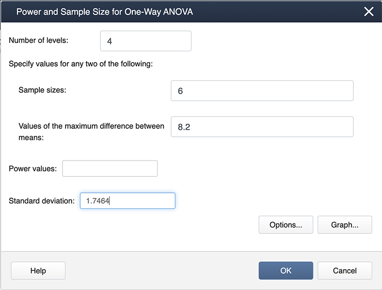
Figure \(\PageIndex{b2}\): Entering values in the Power and Sample Size pop-up window.

When you look at our filled-in dialogue box, you will notice we have not entered a value for power. This is because Minitab will calculate whichever box you leave blank (so if we needed sample size we would leave sample size blank and fill in a value for power). From our example, we know the number of levels is 4 because we have four treatments. We have six observations for each treatment so the sample size is 6. The value for the maximum difference in the means is 8.2 (we simply subtracted the smallest mean from the largest mean, and the standard deviation is 1.747. Where did this come from? The MSE, available from the ANOVA table, is about 3, and hence the standard deviation is \(\sqrt{3}=1.747\)).

After we click OK we get the following output:

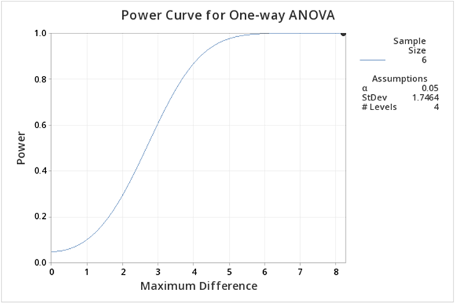
Figure \(\PageIndex{b3}\): Power curve for greenhouse data one-way ANOVA, with 4 treatment levels.

If you follow this graph you see that power is on the y-axis and the power for the specific setting is indicated by a red dot. It is hard to find, but if you look carefully the red dot corresponds to a power of 1. In practice, this is very unusual, but can be easily explained given that the greenhouse data was constructed to show differences.

We can ask the question, what about differences among the treatment groups, not considering the control? All we need to do is modify some of the input in Minitab.

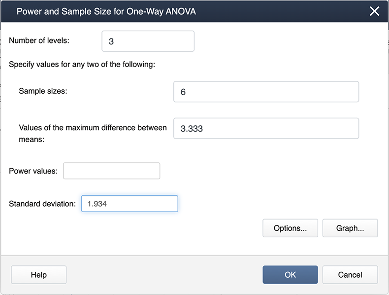
Figure \(\PageIndex{b4}\): Entering modified values in the Power and Sample Size window.

Note the differences here as in the previous screenshot. We now have 3 levels because we are only considering the three treatments. The maximum differences among the means and also the standard deviation are also different.

The output now is much easier to see:

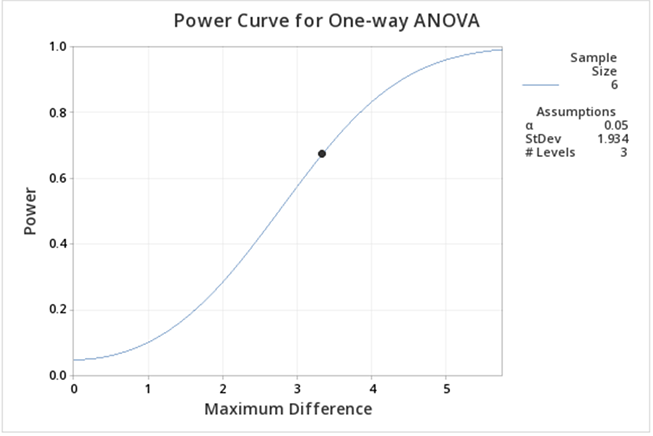
Figure \(\PageIndex{b5}\): Power curve for greenhouse data one-way ANOVA, with 3 treatment levels (control omitted).

Here we can see the power is lower than when including the control. The main reason for this decrease is that the difference between the means is smaller.

You can experiment with the power function in Minitab to provide you with sample sizes, etc. for various powers. Below is some sample output when we ask for various power curves for various sample sizes, a kind of "what if" scenario.

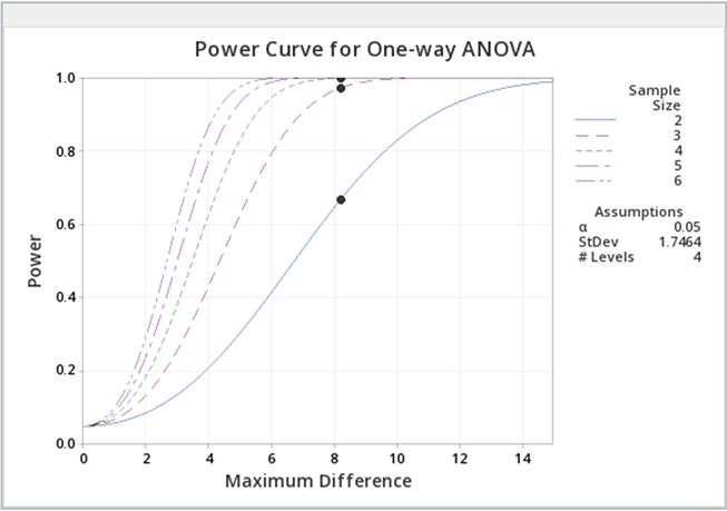
Figure \(\PageIndex{b6}\): Power curves for greenhouse data, with varying sample sizes.

Just as a reminder, power analyses are most often performed BEFORE an experiment is conducted, but occasionally, a power analysis can provide some evidence as to why significant differences were not found.

Using R

Steps in R

With the following commands we will get the power analysis for the greenhouse example:

groupmeans<-c(21,28.6,25.87,29.2)
power.anova.test(groups=4,n=6,between.var=var(groupmeans),within.var=3.05,sig.level=0.05)
Balanced one-way analysis of variance power calculation
groups = 4
n = 6
between.var = 13.96823
within.var = 3.05
sig.level = 0.05
power = 1

NOTE: n is the number in each group.

If we want to produce a power plot by increasing the sample size and the variance (like the one produced by SAS) we can use the following commands:

groupmeans<-c(21,28.6,25.87,29.2)
n<-c(seq(2,8,by=1))
p<power.anova.test(groups=4,n=n,between.var=var(groupmeans),within.var=3.05,sig.level=0.05)
p1<power.anova.test(groups=4,n=n,between.var=var(groupmeans),within.var=4,sig.level=0.05)
p2<power.anova.test(groups=4,n=n,between.var=var(groupmeans),within.var=6.25,sig.level=0.05)
p3<power.anova.test(groups=4,n=n,between.var=var(groupmeans),within.var=9,sig.level=0.05)
p4<power.anova.test(groups=4,n=n,between.var=var(groupmeans),within.var=16.05,sig.level=0.05)
p5<power.anova.test(groups=4,n=n,between.var=var(groupmeans),within.var=25,sig.level=0.05)
plot(n,p$power,ylab="Power",xlab="Sample size per group",main="Overall F test for One-Way ANOVA", ylim=c(0,1))
lines(n,p$power, col = "blue")
abline(h=0.80)
par(new=TRUE)
plot(n,p1$power,ylab="Power",xlab="Sample size per group",main="Overall F test for One-Way ANOVA",ylim=c(0,1))
lines(n,p1$power, col = "red")
par(new=TRUE)
plot(n,p2$power,ylab="Power",xlab="Sample size per group",main="Overall F test for One-Way ANOVA",ylim=c(0,1))
lines(n,p2$power, col = "green")
par(new=TRUE)
plot(n,p3$power,ylab="Power",xlab="Sample size per group",main="Overall F test for One-Way ANOVA",ylim=c(0,1))
lines(n,p3$power, col = "brown")
par(new=TRUE)
plot(n,p4$power,ylab="Power",xlab="Sample size per group",main="Overall F test for One-Way ANOVA",ylim=c(0,1))
lines(n,p4$power, col = "purple")
par(new=TRUE)
plot(n,p5$power,ylab="Power",xlab="Sample size per group",main="Overall F test for One-Way ANOVA",ylim=c(0,1))
lines(n,p5$power, col = "gray")
text(locator(1),"var=3.05",col="blue")
text(locator(1),"var=4",col="red")
text(locator(1),"var=6.25",col="green")
text(locator(1),"var=9",col="brown")
text(locator(1),"var=16",col="purple")
text(locator(1),"var=25",col="gray")

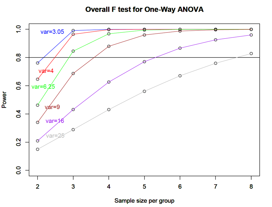
Figure \(\PageIndex{c1}\): Plot of overall \(F\)-test for one-way ANOVA of greenhouse data.