
16.2.1: Critical Values of Chi-Square Table
- Page ID
- 18948

\( \newcommand{\vecs}[1]{\overset { \scriptstyle \rightharpoonup} {\mathbf{#1}} } \)
\( \newcommand{\vecd}[1]{\overset{-\!-\!\rightharpoonup}{\vphantom{a}\smash {#1}}} \)
\( \newcommand{\id}{\mathrm{id}}\) \( \newcommand{\Span}{\mathrm{span}}\)
( \newcommand{\kernel}{\mathrm{null}\,}\) \( \newcommand{\range}{\mathrm{range}\,}\)
\( \newcommand{\RealPart}{\mathrm{Re}}\) \( \newcommand{\ImaginaryPart}{\mathrm{Im}}\)
\( \newcommand{\Argument}{\mathrm{Arg}}\) \( \newcommand{\norm}[1]{\| #1 \|}\)
\( \newcommand{\inner}[2]{\langle #1, #2 \rangle}\)
\( \newcommand{\Span}{\mathrm{span}}\)
\( \newcommand{\id}{\mathrm{id}}\)
\( \newcommand{\Span}{\mathrm{span}}\)
\( \newcommand{\kernel}{\mathrm{null}\,}\)
\( \newcommand{\range}{\mathrm{range}\,}\)
\( \newcommand{\RealPart}{\mathrm{Re}}\)
\( \newcommand{\ImaginaryPart}{\mathrm{Im}}\)
\( \newcommand{\Argument}{\mathrm{Arg}}\)
\( \newcommand{\norm}[1]{\| #1 \|}\)
\( \newcommand{\inner}[2]{\langle #1, #2 \rangle}\)
\( \newcommand{\Span}{\mathrm{span}}\) \( \newcommand{\AA}{\unicode[.8,0]{x212B}}\)
\( \newcommand{\vectorA}[1]{\vec{#1}} % arrow\)
\( \newcommand{\vectorAt}[1]{\vec{\text{#1}}} % arrow\)
\( \newcommand{\vectorB}[1]{\overset { \scriptstyle \rightharpoonup} {\mathbf{#1}} } \)
\( \newcommand{\vectorC}[1]{\textbf{#1}} \)
\( \newcommand{\vectorD}[1]{\overrightarrow{#1}} \)
\( \newcommand{\vectorDt}[1]{\overrightarrow{\text{#1}}} \)
\( \newcommand{\vectE}[1]{\overset{-\!-\!\rightharpoonup}{\vphantom{a}\smash{\mathbf {#1}}}} \)
\( \newcommand{\vecs}[1]{\overset { \scriptstyle \rightharpoonup} {\mathbf{#1}} } \)
\( \newcommand{\vecd}[1]{\overset{-\!-\!\rightharpoonup}{\vphantom{a}\smash {#1}}} \)
\(\newcommand{\avec}{\mathbf a}\) \(\newcommand{\bvec}{\mathbf b}\) \(\newcommand{\cvec}{\mathbf c}\) \(\newcommand{\dvec}{\mathbf d}\) \(\newcommand{\dtil}{\widetilde{\mathbf d}}\) \(\newcommand{\evec}{\mathbf e}\) \(\newcommand{\fvec}{\mathbf f}\) \(\newcommand{\nvec}{\mathbf n}\) \(\newcommand{\pvec}{\mathbf p}\) \(\newcommand{\qvec}{\mathbf q}\) \(\newcommand{\svec}{\mathbf s}\) \(\newcommand{\tvec}{\mathbf t}\) \(\newcommand{\uvec}{\mathbf u}\) \(\newcommand{\vvec}{\mathbf v}\) \(\newcommand{\wvec}{\mathbf w}\) \(\newcommand{\xvec}{\mathbf x}\) \(\newcommand{\yvec}{\mathbf y}\) \(\newcommand{\zvec}{\mathbf z}\) \(\newcommand{\rvec}{\mathbf r}\) \(\newcommand{\mvec}{\mathbf m}\) \(\newcommand{\zerovec}{\mathbf 0}\) \(\newcommand{\onevec}{\mathbf 1}\) \(\newcommand{\real}{\mathbb R}\) \(\newcommand{\twovec}[2]{\left[\begin{array}{r}#1 \\ #2 \end{array}\right]}\) \(\newcommand{\ctwovec}[2]{\left[\begin{array}{c}#1 \\ #2 \end{array}\right]}\) \(\newcommand{\threevec}[3]{\left[\begin{array}{r}#1 \\ #2 \\ #3 \end{array}\right]}\) \(\newcommand{\cthreevec}[3]{\left[\begin{array}{c}#1 \\ #2 \\ #3 \end{array}\right]}\) \(\newcommand{\fourvec}[4]{\left[\begin{array}{r}#1 \\ #2 \\ #3 \\ #4 \end{array}\right]}\) \(\newcommand{\cfourvec}[4]{\left[\begin{array}{c}#1 \\ #2 \\ #3 \\ #4 \end{array}\right]}\) \(\newcommand{\fivevec}[5]{\left[\begin{array}{r}#1 \\ #2 \\ #3 \\ #4 \\ #5 \\ \end{array}\right]}\) \(\newcommand{\cfivevec}[5]{\left[\begin{array}{c}#1 \\ #2 \\ #3 \\ #4 \\ #5 \\ \end{array}\right]}\) \(\newcommand{\mattwo}[4]{\left[\begin{array}{rr}#1 \amp #2 \\ #3 \amp #4 \\ \end{array}\right]}\) \(\newcommand{\laspan}[1]{\text{Span}\{#1\}}\) \(\newcommand{\bcal}{\cal B}\) \(\newcommand{\ccal}{\cal C}\) \(\newcommand{\scal}{\cal S}\) \(\newcommand{\wcal}{\cal W}\) \(\newcommand{\ecal}{\cal E}\) \(\newcommand{\coords}[2]{\left\{#1\right\}_{#2}}\) \(\newcommand{\gray}[1]{\color{gray}{#1}}\) \(\newcommand{\lgray}[1]{\color{lightgray}{#1}}\) \(\newcommand{\rank}{\operatorname{rank}}\) \(\newcommand{\row}{\text{Row}}\) \(\newcommand{\col}{\text{Col}}\) \(\renewcommand{\row}{\text{Row}}\) \(\newcommand{\nul}{\text{Nul}}\) \(\newcommand{\var}{\text{Var}}\) \(\newcommand{\corr}{\text{corr}}\) \(\newcommand{\len}[1]{\left|#1\right|}\) \(\newcommand{\bbar}{\overline{\bvec}}\) \(\newcommand{\bhat}{\widehat{\bvec}}\) \(\newcommand{\bperp}{\bvec^\perp}\) \(\newcommand{\xhat}{\widehat{\xvec}}\) \(\newcommand{\vhat}{\widehat{\vvec}}\) \(\newcommand{\uhat}{\widehat{\uvec}}\) \(\newcommand{\what}{\widehat{\wvec}}\) \(\newcommand{\Sighat}{\widehat{\Sigma}}\) \(\newcommand{\lt}{<}\) \(\newcommand{\gt}{>}\) \(\newcommand{\amp}{&}\) \(\definecolor{fillinmathshade}{gray}{0.9}\)A new type of statistical analysis, a new table of critical values!
Chi-Square Distributions
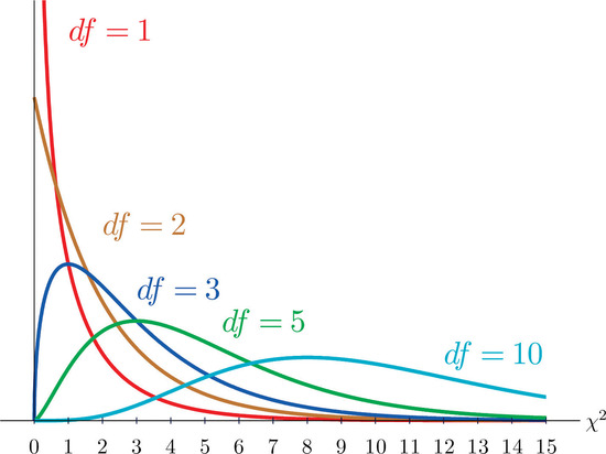
As you know, there is a whole family of \(t\)-distributions, each one specified by a parameter called the degrees of freedom (\(df\)). Similarly, all the chi-square distributions form a family, and each of its members is also specified by a its own \(df\). Chi (like "kite," not like "chai" or "Chicago") is a Greek letter denoted by the symbol \(\chi\) and chi-square is often denoted by \(\chi^2\). It looks like a wiggly X, but is not an X. Figure \(\PageIndex{1}\) shows several \(\chi\)-square distributions for different degrees of freedom.
Like all tables of critical values, this one provides the value in which you should reject the null hypothesis if your calculated value is bigger than the critical value i the table. For chi-square, the null hypothesis is that there is no pattern of relationship, but the process of Null Hypothesis Signficance Testing is the same as we've been learning.
Note
Critical < Calculated == Reject null == There is a pattern of relationship. == p<.05
Critical > Calculated == Retain null == There is no pattern of relationship. == p>.05
Illustrated in Figure \(\PageIndex{2}\), the value of the chi-square that cuts off a right tail of area \(c\) is denoted \(\chi_c^2\) and is called a critical value (Figure \(\PageIndex{2}\)).
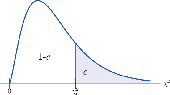
Table of Critical Values for \(\chi_c^2\)
Table \(\PageIndex{1}\) below gives values of \(\chi_c^2\) for various values of \(c\) and under several chi-square distributions with various degrees of freedom.
| df | p = 0.10 | p = 0.05 | p = 0.01 |
|---|---|---|---|
| 1 | 2.706 | 3.841 | 6.635 |
| 2 | 4.605 | 5.991 | 9.210 |
| 3 | 6.251 | 7.815 | 11.345 |
| 4 | 7.779 | 9.488 | 13.277 |
| 5 | 9.236 | 11.070 | 15.086 |
| 6 | 10.645 | 12.592 | 16.812 |
| 7 | 12.017 | 14.067 | 18.475 |
| 8 | 13.362 | 15.507 | 20.090 |
| 9 | 14.684 | 16.919 | 21.666 |
| 10 | 15.987 | 18.307 | 23.209 |
| 11 | 17.275 | 19.675 | 24.725 |
| 12 | 18.549 | 21.026 | 26.217 |
| 13 | 19.812 | 22.362 | 27.688 |
| 14 | 21.064 | 23.685 | 29.141 |
| 15 | 22.307 | 24.996 | 30.578 |
| 16 | 23.542 | 26.296 | 32.000 |
| 17 | 24.769 | 27.587 | 33.409 |
| 18 | 25.989 | 28.869 | 34.805 |
| 19 | 27.204 | 30.144 | 36.191 |
| 20 | 28.412 | 31.410 | 37.566 |
| 100 | 118.498 | 124.342 | 135.807 |
Degrees of Freedom
Like with the t-test and ANOVA, the degrees of freedom are based on which kind of analysis you are conducting.
- \(\chi_{GoF}^2\) Goodness of Fit: \(k-1\)
- k is the number of categories.
- \(\chi_{ToI}^2\) Test of Independence: \((R-1)\times(C-1) \)
- R is the number of rows
- C is the number of columns
- Kruskal-Wallis Test: \(k-1 \)
- k is the number of groups