3.5: Graphs and Properties of Logarithmic Functions

Last updated
Save as PDF

Page ID: 26515

$ \newcommand{\vecs}[1]{\overset { \scriptstyle \rightharpoonup} {\mathbf{#1}} } $ $ \newcommand{\vecd}[1]{\overset{-\!-\!\rightharpoonup}{\vphantom{a}\smash {#1}}} $$\newcommand{\id}{\mathrm{id}}$ $ \newcommand{\Span}{\mathrm{span}}$ $ \newcommand{\kernel}{\mathrm{null}\,}$ $ \newcommand{\range}{\mathrm{range}\,}$ $ \newcommand{\RealPart}{\mathrm{Re}}$ $ \newcommand{\ImaginaryPart}{\mathrm{Im}}$ $ \newcommand{\Argument}{\mathrm{Arg}}$ $ \newcommand{\norm}[1]{\| #1 \|}$ $ \newcommand{\inner}[2]{\langle #1, #2 \rangle}$ $ \newcommand{\Span}{\mathrm{span}}$ $\newcommand{\id}{\mathrm{id}}$ $ \newcommand{\Span}{\mathrm{span}}$ $ \newcommand{\kernel}{\mathrm{null}\,}$ $ \newcommand{\range}{\mathrm{range}\,}$ $ \newcommand{\RealPart}{\mathrm{Re}}$ $ \newcommand{\ImaginaryPart}{\mathrm{Im}}$ $ \newcommand{\Argument}{\mathrm{Arg}}$ $ \newcommand{\norm}[1]{\| #1 \|}$ $ \newcommand{\inner}[2]{\langle #1, #2 \rangle}$ $ \newcommand{\Span}{\mathrm{span}}$$\newcommand{\AA}{\unicode[.8,0]{x212B}}$

Learning Objectives

In this section, you will:

examine properties of logarithmic functions
examine graphs of logarithmic functions
examine the relationship between graphs of exponential and logarithmic functions

Recall that the exponential function $f(x) = 2^x$ produces this table of values

$x$	-3	-2	-1	0	1	2	3
$f(x)$	1/8	1/4	1/2	1	2	4	8

Since the logarithmic function is an inverse of the exponential, $g(x)=\log_{2}(x)$ produces the table of values

$x$	1/8	1/4	1/2	1	2	4	8
$g(x)$	-3	-2	-1	0	1	2	3

In this second table, notice that

As the input increases, the output increases.
As input increases, the output increases more slowly.
Since the exponential function only outputs positive values, the logarithm can only accept positive values as inputs, so the domain of the log function is $(0, \infty)$.
Since the exponential function can accept all real numbers as inputs, the logarithm can have any real number as output, so the range is all real numbers or $(-\infty, \infty)$.

$5.5.png$

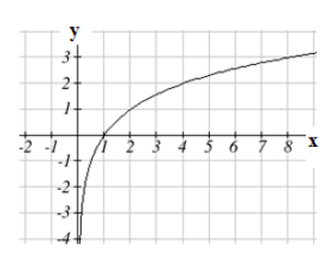
Plotting the graph of $g(x) = \log_{2}(x)$ from the points in the table , notice that as the input values for $x$ approach zero, the output of the function grows very large in the negative direction, indicating a vertical asymptote at $x = 0$.

In symbolic notation we write

as $x \rightarrow 0^{+}$, $f(x) \rightarrow-\infty$

and as $x \rightarrow \infty, f(x) \rightarrow \infty$

Source: The material in this section of the textbook originates from David Lippman and Melonie Rasmussen, Open Text Bookstore, Precalculus: An Investigation of Functions, “Chapter 4: Exponential and Logarithmic Functions,” licensed under a Creative Commons CC BY-SA 3.0 license. The material here is based on material contained in that textbook but has been modified by Roberta Bloom, as permitted under this license.

Graphically, in the function $g(x) = \log_{b}(x)$, $b > 1$, we observe the following properties:

$5.5b.png$

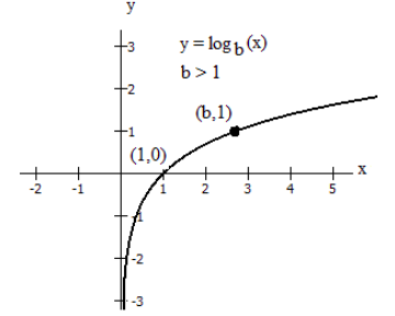
The graph has a horizontal intercept at (1, 0)
The line x = 0 (the y-axis) is a vertical asymptote; as $x \rightarrow 0^{+}, y \rightarrow-\infty$
The graph is increasing if $b > 1$
The domain of the function is $x > 0$, or (0, $\infty$)
The range of the function is all real numbers, or $(-\infty, \infty)$

However if the base $b$ is less than 1, 0 < $b$ < 1, then the graph appears as below.
This follows from the log property of reciprocal bases : $\log _{1 / b} C=-\log _{b}(C)$

$5.5c.png$

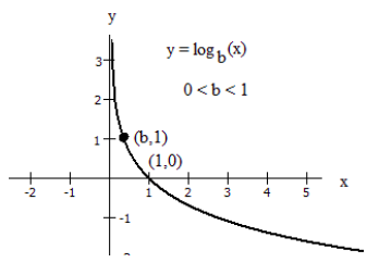
The graph has a horizontal intercept at (1, 0)
The line x = 0 (the y-axis) is a vertical asymptote; as $x \rightarrow 0^{+}, y \rightarrow \infty$
The graph is decreasing if 0 < $b$ < 1
The domain of the function is $x$ > 0, or (0, $\infty$)
The range of the function is all real numbers, or $(-\infty, \infty)$

When graphing a logarithmic function, it can be helpful to remember that the graph will pass through the points (1, 0) and ($b$, 1).

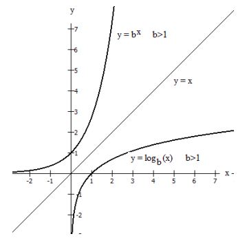
Finally, we compare the graphs of $y = b^x$ and $y = \log_{b}(x)$, shown below on the same axes.

Because the functions are inverse functions of each other, for every specific ordered pair
($h$, $k$) on the graph of $y = b^x$, we find the point ($k$, $h$) with the coordinates reversed on the graph of $y = \log_{b}(x)$.

In other words, if the point with $x = h$ and $y = k$ is on the graph of $y = b^x$, then the point with $x = k$ and $y = h$ lies on the graph of $y = \log_{b} (x)$

The domain of $y = b^x$ is the range of $y = \log_{b} (x)$

The range of $y = b^x$ is the domain of $y = \log_{b} (x)$

For this reason, the graphs appear as reflections, or mirror images, of each other across the diagonal line $y=x$. This is a property of graphs of inverse functions that students should recall from their study of inverse functions in their prerequisite algebra class.

$5.5d.png$

	$\bf{y = b^x}$, with $\bf{b>1}$	$\bf{y = \log_{b} (x)}$, with $\bf{b>1}$
Domain	1}\)" valign="top" width="188" class="lt-math-38599"> all real numbers	1}\)" valign="top" width="189" class="lt-math-38599"> all positive real numbers
Range	1}\)" valign="top" width="188" class="lt-math-38599"> all positive real numbers	1}\)" valign="top" width="189" class="lt-math-38599"> all real numbers
Intercepts	1}\)" valign="top" width="188" class="lt-math-38599"> (0,1)	1}\)" valign="top" width="189" class="lt-math-38599"> (1,0)
Asymptotes	1}\)" valign="top" width="188" class="lt-math-38599"> Horizontal asymptote is the line y = 0 (the x-axis) As $x \rightarrow-\infty, \: y \rightarrow 0$	1}\)" valign="top" width="189" class="lt-math-38599"> Vertical asymptote is the line x = 0 (the y axis) As $x \rightarrow 0^{+}, \: y \rightarrow-\infty$