7.4: Confidence Interval for Standard Deviation

When you open a bag of dog kibble, there is an expectation of how much is in the bag. Kibble filling machines do not necessarily fill each bag to the exact weight on the label, there may be a bit more or even a little bit less. In instances like this, we would be interested in checking if a filling machine is consistent in its filling capabilities. Examples like this measure consistency (i.e., how spread out are the data values); thus, in this section, we will discuss how to construct confidence intervals for a population standard deviation.

Recall, to find the confidence interval for a population proportion, you used the normal distribution and to find the confidence interval for population mean, you used the Student's \( t\)-distribution. In this section, we will need to introduce a new distribution called the \( \chi^2 \) distribution, which we will use a table.

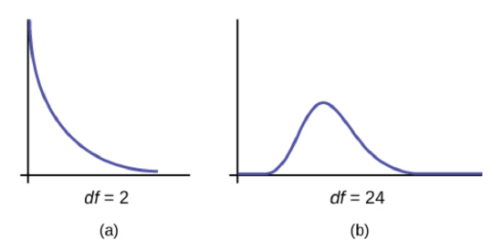
First, the \( \chi^2 \) distribution curve is not symmetrical and depends on the degree of freedom ( \( df = n-1 \) ). The smaller the degree of free, the curve looks more skewed right. The bigger the degree of freedom, the curve looks more symmetric.

Figure 7.4.1

Second, \( \chi^2 \)-distribution table relies on the degree of freedom ( \( df =n-1 \) ) and the area in the right tail. In the table, the first column gives to the degree of freedom. The first row indicates the subscript value for the \( \chi^2\) critical values. This subscript represents the area in the right tail.

Figure 7.4.2

Example 7.4.1

Given \( n=12 \), find \( \chi^2_{0.01} \).

Answer

Notice that \( \alpha\) (the subscript) is \(0.01\). This represents the area in the right tail. Draw a \( \chi^2 \) curve, shade the right tail as 0.01. Since \( n=12\), that means the degree of freedom \(df=11\).

Figure 7.4.3

Under the column labeled as \( 0.01\) and across the row of degree of freedom \( df=12-1=11 \)

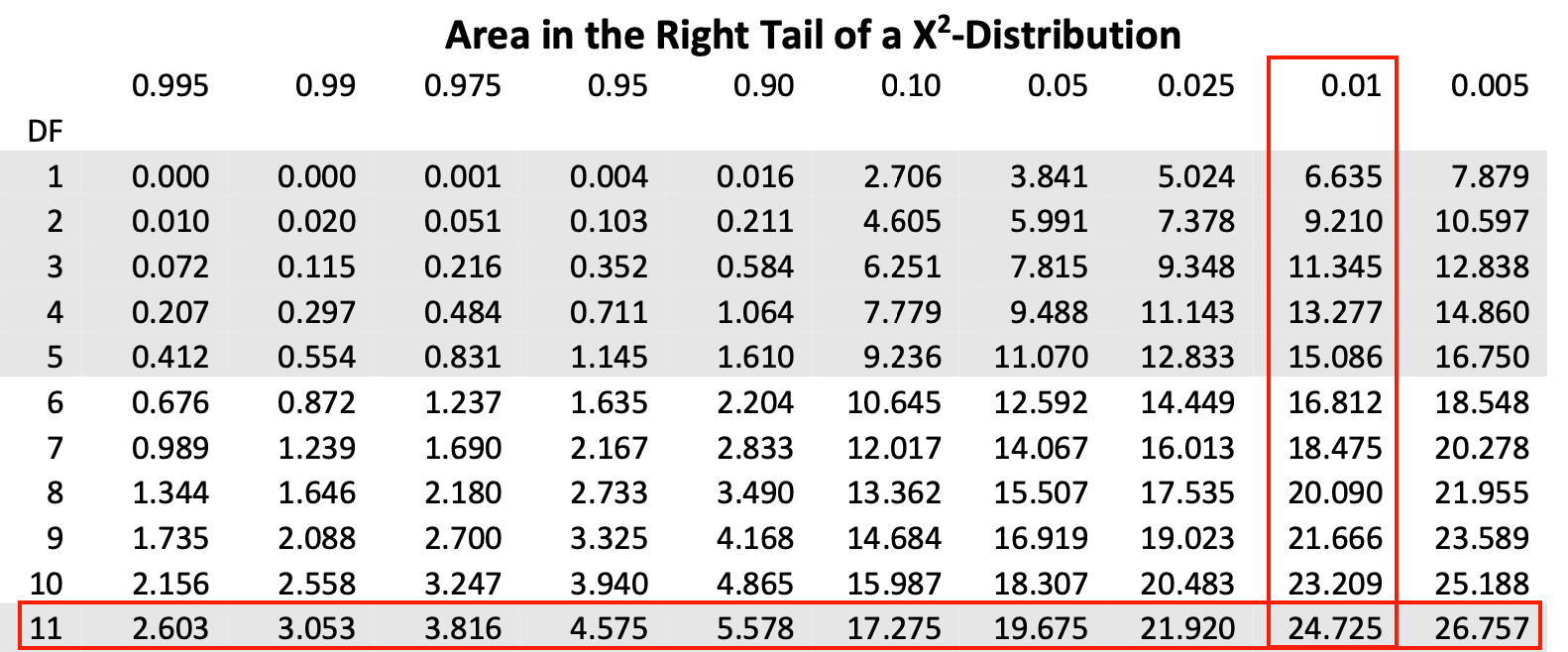
Figure 7.4.4

Thus, we can label that the tail begins at \( \chi^2_{0.01} =24.725\).

Figure 7.4.5

The following is the confidence interval for a population standard deviation:

\[ \sqrt{ \dfrac{(n-1) s^2}{\chi^2_{\alpha/2}} } < \sigma^2 < \sqrt{ \dfrac{(n-1) s^2}{\chi^2_{1-\alpha/2}} } \]

where the lower boundf\( \sqrt{ \dfrac{(n-1) s^2}{\chi^2_{\alpha/2}}} \) and the upper bound = \( \sqrt{ \dfrac{(n-1) s^2}{\chi^2_{1-\alpha/2}}} \)

Requirement: \( X\) is normally distributed.

Notice that the formula does not look like the previous confidence interval format of "point estimate \( \pm \) margin of error." Also, notice that the critical values in the denominators look similar but subscripts are not the same. Let's talk about critical values.

Example 7.4.2

Example 7.4.2

Find the critical values given a \(95 \%\) level of confidence and the sample size \( n= 5 \).

Answer

Given\( n= 5 \), then the degree of freedom \( df= 5-1=4 \). Thus, we will look at the 4th row of the table.

Notice, no \( \alpha\) is explicitly given here. What do we do? To find \( \alpha\), subtract the level of confidence from \(1 \). So, \( \alpha=1-0.95=0.05 \). Which means, \( \alpha/2 = 0.025 \) and \( 1-\alpha/2 = 0.975 \).

To find \( \chi^2_{\alpha/2} \), we will look for \( \chi^2_{0.025} \). To find \(1- \chi^2_{\alpha/2} \), we will look for \( \chi^2_{0.975} \). We look for the subscript value in the top row of the table.

The critical values are \( \chi^2_{0.025} =11.143\) and \( \chi^2_{0.975} =0.484\)

Figure 7.4.6

Figure 7.4.7

In the next example, we will find a confidence interval for population standard deviation.

Example 7.4.3

You buy in bulk 12 bags of dog kibble and weigh each bag. The following data is the weight in pounds.

(a) Find the confidence interval for the standard deviation at a \(90\%\) level of confidence.

(b) Give an interpretation of your confidence interval.

9.63	9.60	8.98	9.86
9.52	9.53	9.78	9.56
9.12	9.25	9.52	9.34

Answers:

(a) First find the critical values. Since \( \alpha = 0.10\), then \( \alpha/2 = 0.05\) and \( 1-\alpha/2 = 0.95\). Looking at the columns labeled \(0.05\) and \(0.95\) with the df row of \(11\), we see that \( \chi^2_{0.05} = 19.675\) and \( \chi^2_{0.95} = 4.575\)

Figure 7.4.8

Now, find the sample standard deviation. The sample standard deviation \( s=0.2585\).

Lastly, putting everything together:

lower bound \(= \sqrt{ \dfrac{(n-1) s^2}{\chi^2_{\alpha/2}}} =\sqrt {\dfrac{ (12-1) 0.2585^2 }{ 19.675} }=0.1933\)

upper bound \(= \sqrt{ \dfrac{(n-1) s^2}{\chi^2_{1-\alpha/2}}} =\sqrt {\dfrac{(12-1) 0.2585^2}{4.575}}=0.4008\)

The confidence interval is \( 0.1933< \sigma < 0.4008 \) pounds. (Notice in this example, we are not moving the decimal to the left twice because these values do not represent percentages, but pounds.)

(b) We are \( 90\%\) confident that the true standard deviation of potato chip bag weight is between \( 0.1933\) and \(0.4008 \) ounces.

Contributors and Attributions

• Barbara Illowsky and Susan Dean (De Anza College) with many other contributing authors. Content produced by OpenStax College is licensed under a Creative Commons Attribution License 4.0 license. Download for free at http://cnx.org/contents/30189442-699...b91b9de@18.114