7.3: Confidence Interval for a Mean

You have determined to turn your dusty backyard into a flower paradise. Before you start any work, you want to know if this idea is worth it. You visit the local park and have noticed that certain flowers do not last for very long after blooming. Seeking scientific proof to make your decision, you have collected data on the number of days you notice the flowers are in full bloom. What should you do with this data?

You can quickly calculate the mean number of days of full bloom. But you have decided that this single number does not determine the range of possible days that a full bloom occurs. To do so, you will need to build a confidence interval for mean.

The following is the confidence interval for a population mean:

$$\bar{x} - t_{\alpha/2} \cdot \dfrac{s}{\sqrt{n}} < \mu < \bar{x} +t_{\alpha/2} \cdot \dfrac{s}{\sqrt{n}}$$

where the lower bound = $\bar{x} - t_{\alpha/2} \cdot \dfrac{s}{\sqrt{n}}$ and the upper bound = $\bar{x} +t_{\alpha/2} \cdot \dfrac{s}{\sqrt{n}}$, and a margin of error = $\bar{x} +t_{\alpha/2} \cdot \dfrac{s}{\sqrt{n}}$.

Requirement: $X$ is normally distributed or $n\geq 30$

Notice, the new notation of $t_{\alpha/2}$. This critical value refers to the Student's t-distribution which is described in more detail below.

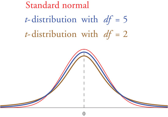
Student’s $t$-distribution with $n-1$ degrees of freedom. Student’s $t$-distribution is very much like the standard normal distribution in that it is centered at $0$ and has the same qualitative bell shape, but it has heavier tails than the standard normal distribution does, as indicated by Figure 7.3.1 , in which the curve (in brown) that meets the dashed vertical line at the lowest point is the $t$-distribution with two degrees of freedom, the next curve (in blue) is the $t$-distribution with five degrees of freedom, and the thin curve (in red) is the standard normal distribution. As also indicated by the figure, as the sample size $n$ increases, Student’s $t$-distribution ever more closely resembles the standard normal distribution. Although there is a different $t$-distribution for every value of $n$, once the sample size is $30$ or more it is typically acceptable to use the standard normal distribution instead, as we will always do in this text.

Figure 7.3.1 : Student’s $t$-DistributionJ

Student's $t$-distribution table relies on the degree of freedom ( $df =n-1$ ) and the area in the right tail. In the table, the first column gives to the degree of freedom. The first row indicates the subscript value for the Student's $t$ critical values. This subscript represents the area in the right tail.

Example 7.3.1

Use Figure 7.3.1 below to find the number $t_{\alpha /2}$ needed in construction of a confidence interval:

1. when the level of confidence is $90\%$ with $n=15$
2. when the level of confidence is $99\%$ with $n=23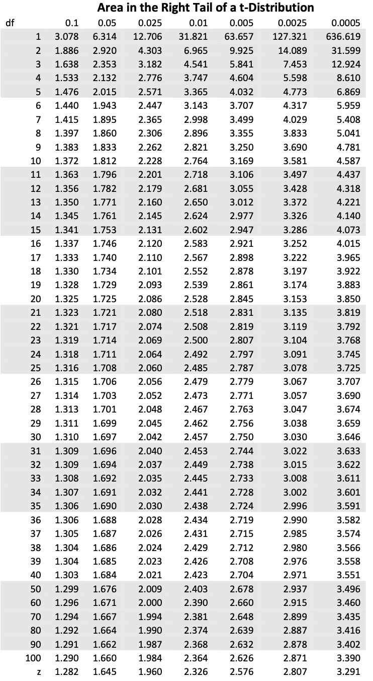$ Figure 7.3.1 : Critical Values of t

Solution:

1. Figure 7.3.1 gives the critical values which is the cut-off value for which area in the right tail. The area in the right tail is defined by $\alpha/2$. We will start with finding $\alpha$, which is $1- \text{ confidence level } = 1 - 0.90= 0.10$. Now to get $\alpha/2$, we divide $0.10$ by 2. So, $\alpha/2=0.05$, which is the column we In other words, we need to find $t_{0.05}$. The subscript $0.05$ is the column which we will look under. And, we will look at the degree of freedom$=n-1$ row. In this example our degree of freedom is $14$ (because $15-1$). Thus, $t_{0.05}=1.761$.
2. In Figure 7.3.1 $t_{0.005}$ is the number in the 22nd row and in the column headed ${0.005}$, namely $2.819$.

Example 7.3.2

A sample of size $15$ drawn from a normally distributed population has sample mean $35$ and sample standard deviation $14$. Construct a $95\%$ confidence interval for the population mean, and interpret its meaning.

Solution:

Since the population is normally distributed, the sample is small, and the population standard deviation is unknown, the formula that applies is Equation $\ref{tdist}$.

Confidence level $95\%$ means that

$$α=1−0.95=0.05$$

so $α/2=0.025$. Since the sample size is $n = 15$, there are $n−1=14$ degrees of freedom. By Figure 7.1.6 $t_{0.025}=2.145$. Thus

$$\begin{align} \overline{x} &= ±t_{α/2} \left( \dfrac{s}{\sqrt{n}}\right) \\ &=35 ± 2.145 \left( \dfrac{14}{\sqrt{15}} \right) \\ &=35 ±7.8 \end{align}$$

One may be $95\%$ confident that the true value of $μ$ is contained in the interval

$$(35−7.8, 35+7.8) = (27.2,42.8).$$

Example 7.3.3

A random sample of $12$ students from a large university yields mean GPA $2.71$ with sample standard deviation $0.51$. Construct a $90\%$ confidence interval for the mean GPA of all students at the university. Assume that the numerical population of GPAs from which the sample is taken has a normal distribution.

Solution:

Since the population is normally distributed, the sample is small, and the population standard deviation is unknown, the formula that applies is Equation $\ref{tdist}$

Confidence level $90\%$ means that

$$α=1−0.90=0.10$$

so $α/2=0.05$. Since the sample size is $n = 12$, there are $n−1=11$ degrees of freedom. By Figure 7.1.6 $t_{0.05}=1.796$. Thus

$$\begin{align} \overline{x} &= ±t_{α/2} \left( \dfrac{s}{\sqrt{n}}\right) \\ &=2.71 ± 1.796 \left( \dfrac{0.51}{\sqrt{12}} \right) \\ &=2.71 ±0.26 \end{align}$$

AutoAttribution

• 7.2: Small Sample Estimation of a Population Mean, is licensed CC BY-NC-SA