7.2: Small Sample Estimation of a Population Mean

Learning Objectives

1. To become familiar with Student’s $t$-distribution.
2. To understand how to apply additional formulas for a confidence interval for a population mean.

The confidence interval formulas in the previous section are based on the Central Limit Theorem, the statement that for large samples $\overline{X}$ is normally distributed with mean $\mu$ and standard deviation $\sigma /\sqrt{n}$. When the population mean $\mu$ is estimated with a small sample ($n<30$), the Central Limit Theorem does not apply. In order to proceed we assume that the numerical population from which the sample is taken has a normal distribution to begin with. If this condition is satisfied then when the population standard deviation $\sigma$ is known the old formula $\bar{x}\pm z_{\alpha /2}(\sigma /\sqrt{n})$ can still be used to construct a $100(1-\alpha )\%$ confidence interval for $\mu$.

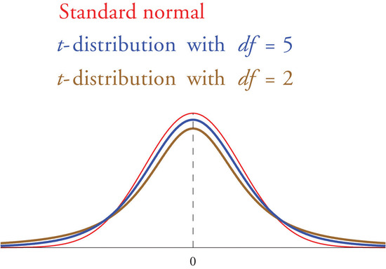
If the population standard deviation is unknown and the sample size $n$ is small then when we substitute the sample standard deviation $s$ for $\sigma$ the normal approximation is no longer valid. The solution is to use a different distribution, called Student’s $t$-distribution with $n-1$ degrees of freedom. Student’s $t$-distribution is very much like the standard normal distribution in that it is centered at $0$ and has the same qualitative bell shape, but it has heavier tails than the standard normal distribution does, as indicated by Figure $\PageIndex{1}$, in which the curve (in brown) that meets the dashed vertical line at the lowest point is the $t$-distribution with two degrees of freedom, the next curve (in blue) is the $t$-distribution with five degrees of freedom, and the thin curve (in red) is the standard normal distribution. As also indicated by the figure, as the sample size $n$ increases, Student’s $t$-distribution ever more closely resembles the standard normal distribution. Although there is a different $t$-distribution for every value of $n$, once the sample size is $30$ or more it is typically acceptable to use the standard normal distribution instead, as we will always do in this text.

Figure $\PageIndex{1}$: Student’s $t$-Distribution

Just as the symbol $z_c$ stands for the value that cuts off a right tail of area $c$ in the standard normal distribution, so the symbol $t_c$ stands for the value that cuts off a right tail of area $c$ in the standard normal distribution. This gives us the following confidence interval formulas.

Small Sample $100(1−α)\%$ Confidence Interval for a Population Mean

If $σ$ is known:

$$\overline{x} ±z_{α/2} \left( \dfrac{σ}{\sqrt{n}}\right) \nonumber$$

If $σ$ is unknown:

$$\overline{x} ±t_{α/2} \left( \dfrac{s}{\sqrt{n}}\right) \label{tdist}$$

with the degrees of freedom $df=n−1$.

The population must be normally distributed and a sample is considered small when $n < 30$.

To use the new formula we use the line in Figure 7.1.6 that corresponds to the relevant sample size.

Example $\PageIndex{1}$

A sample of size $15$ drawn from a normally distributed population has sample mean $35$ and sample standard deviation $14$. Construct a $95\%$ confidence interval for the population mean, and interpret its meaning.

Solution

Since the population is normally distributed, the sample is small, and the population standard deviation is unknown, the formula that applies is Equation $\ref{tdist}$.

Confidence level $95\%$ means that

$$α=1−0.95=0.05 \nonumber$$

so $α/2=0.025$. Since the sample size is $n = 15$, there are $n−1=14$ degrees of freedom. By Figure 7.1.6 $t_{0.025}=2.145$. Thus

$$\begin{align} \overline{x}  ±t_{α/2} \left( \dfrac{s}{\sqrt{n}}\right) \\ &=35 ± 2.145 \left( \dfrac{14}{\sqrt{15}} \right) \\ &=35 ±7.8 \end{align} \nonumber$$

One may be $95\%$ confident that the true value of $μ$ is contained in the interval

$$(35−7.8, 35+7.8) = (27.2,42.8). \nonumber$$

Example $\PageIndex{2}$

A random sample of $12$ students from a large university yields mean GPA $2.71$ with sample standard deviation $0.51$. Construct a $90\%$ confidence interval for the mean GPA of all students at the university. Assume that the numerical population of GPAs from which the sample is taken has a normal distribution.

Solution

Since the population is normally distributed, the sample is small, and the population standard deviation is unknown, the formula that applies is Equation $\ref{tdist}$

Confidence level $90\%$ means that

$$α=1−0.90=0.10 \nonumber$$

so $α/2=0.05$. Since the sample size is $n = 12$, there are $n−1=11$ degrees of freedom. By Figure 7.1.6 $t_{0.05}=1.796$. Thus

$$\begin{align} \overline{x}  ±t_{α/2} \left( \dfrac{s}{\sqrt{n}}\right) \\ &=2.71 ± 1.796 \left( \dfrac{0.51}{\sqrt{12}} \right) \\ &=2.71 ±0.26 \end{align} \nonumber$$

One may be $90\%$ confident that the true average GPA of all students at the university is contained in the interval

$$(2.71−0.26,2.71+0.26)=(2.45,2.97). \nonumber$$

Compare "Example 4" in Section 7.1 and "Example 6" in Section 7.1. The summary statistics in the two samples are the same, but the $90\%$ confidence interval for the average GPA of all students at the university in "Example 4" in Section 7.1, $(2.63,2.79)$, is shorter than the $90\%$ confidence interval $(2.45,2.97)$, in "Example 6" in Section 7.1. This is partly because in "Example 4" in Section 7.1 the sample size is larger; there is more information pertaining to the true value of $\mu$ in the large data set than in the small one.

Key Takeaway

• In selecting the correct formula for construction of a confidence interval for a population mean ask two questions: is the population standard deviation $\sigma$ known or unknown, and is the sample large or small?
• We can construct confidence intervals with small samples only if the population is normal.