
7.1: Large Sample Estimation of a Population Mean
- Page ID
- 563
\( \newcommand{\vecs}[1]{\overset { \scriptstyle \rightharpoonup} {\mathbf{#1}} } \)
\( \newcommand{\vecd}[1]{\overset{-\!-\!\rightharpoonup}{\vphantom{a}\smash {#1}}} \)
\( \newcommand{\id}{\mathrm{id}}\) \( \newcommand{\Span}{\mathrm{span}}\)
( \newcommand{\kernel}{\mathrm{null}\,}\) \( \newcommand{\range}{\mathrm{range}\,}\)
\( \newcommand{\RealPart}{\mathrm{Re}}\) \( \newcommand{\ImaginaryPart}{\mathrm{Im}}\)
\( \newcommand{\Argument}{\mathrm{Arg}}\) \( \newcommand{\norm}[1]{\| #1 \|}\)
\( \newcommand{\inner}[2]{\langle #1, #2 \rangle}\)
\( \newcommand{\Span}{\mathrm{span}}\)
\( \newcommand{\id}{\mathrm{id}}\)
\( \newcommand{\Span}{\mathrm{span}}\)
\( \newcommand{\kernel}{\mathrm{null}\,}\)
\( \newcommand{\range}{\mathrm{range}\,}\)
\( \newcommand{\RealPart}{\mathrm{Re}}\)
\( \newcommand{\ImaginaryPart}{\mathrm{Im}}\)
\( \newcommand{\Argument}{\mathrm{Arg}}\)
\( \newcommand{\norm}[1]{\| #1 \|}\)
\( \newcommand{\inner}[2]{\langle #1, #2 \rangle}\)
\( \newcommand{\Span}{\mathrm{span}}\) \( \newcommand{\AA}{\unicode[.8,0]{x212B}}\)
\( \newcommand{\vectorA}[1]{\vec{#1}} % arrow\)
\( \newcommand{\vectorAt}[1]{\vec{\text{#1}}} % arrow\)
\( \newcommand{\vectorB}[1]{\overset { \scriptstyle \rightharpoonup} {\mathbf{#1}} } \)
\( \newcommand{\vectorC}[1]{\textbf{#1}} \)
\( \newcommand{\vectorD}[1]{\overrightarrow{#1}} \)
\( \newcommand{\vectorDt}[1]{\overrightarrow{\text{#1}}} \)
\( \newcommand{\vectE}[1]{\overset{-\!-\!\rightharpoonup}{\vphantom{a}\smash{\mathbf {#1}}}} \)
\( \newcommand{\vecs}[1]{\overset { \scriptstyle \rightharpoonup} {\mathbf{#1}} } \)
\( \newcommand{\vecd}[1]{\overset{-\!-\!\rightharpoonup}{\vphantom{a}\smash {#1}}} \)
\(\newcommand{\avec}{\mathbf a}\) \(\newcommand{\bvec}{\mathbf b}\) \(\newcommand{\cvec}{\mathbf c}\) \(\newcommand{\dvec}{\mathbf d}\) \(\newcommand{\dtil}{\widetilde{\mathbf d}}\) \(\newcommand{\evec}{\mathbf e}\) \(\newcommand{\fvec}{\mathbf f}\) \(\newcommand{\nvec}{\mathbf n}\) \(\newcommand{\pvec}{\mathbf p}\) \(\newcommand{\qvec}{\mathbf q}\) \(\newcommand{\svec}{\mathbf s}\) \(\newcommand{\tvec}{\mathbf t}\) \(\newcommand{\uvec}{\mathbf u}\) \(\newcommand{\vvec}{\mathbf v}\) \(\newcommand{\wvec}{\mathbf w}\) \(\newcommand{\xvec}{\mathbf x}\) \(\newcommand{\yvec}{\mathbf y}\) \(\newcommand{\zvec}{\mathbf z}\) \(\newcommand{\rvec}{\mathbf r}\) \(\newcommand{\mvec}{\mathbf m}\) \(\newcommand{\zerovec}{\mathbf 0}\) \(\newcommand{\onevec}{\mathbf 1}\) \(\newcommand{\real}{\mathbb R}\) \(\newcommand{\twovec}[2]{\left[\begin{array}{r}#1 \\ #2 \end{array}\right]}\) \(\newcommand{\ctwovec}[2]{\left[\begin{array}{c}#1 \\ #2 \end{array}\right]}\) \(\newcommand{\threevec}[3]{\left[\begin{array}{r}#1 \\ #2 \\ #3 \end{array}\right]}\) \(\newcommand{\cthreevec}[3]{\left[\begin{array}{c}#1 \\ #2 \\ #3 \end{array}\right]}\) \(\newcommand{\fourvec}[4]{\left[\begin{array}{r}#1 \\ #2 \\ #3 \\ #4 \end{array}\right]}\) \(\newcommand{\cfourvec}[4]{\left[\begin{array}{c}#1 \\ #2 \\ #3 \\ #4 \end{array}\right]}\) \(\newcommand{\fivevec}[5]{\left[\begin{array}{r}#1 \\ #2 \\ #3 \\ #4 \\ #5 \\ \end{array}\right]}\) \(\newcommand{\cfivevec}[5]{\left[\begin{array}{c}#1 \\ #2 \\ #3 \\ #4 \\ #5 \\ \end{array}\right]}\) \(\newcommand{\mattwo}[4]{\left[\begin{array}{rr}#1 \amp #2 \\ #3 \amp #4 \\ \end{array}\right]}\) \(\newcommand{\laspan}[1]{\text{Span}\{#1\}}\) \(\newcommand{\bcal}{\cal B}\) \(\newcommand{\ccal}{\cal C}\) \(\newcommand{\scal}{\cal S}\) \(\newcommand{\wcal}{\cal W}\) \(\newcommand{\ecal}{\cal E}\) \(\newcommand{\coords}[2]{\left\{#1\right\}_{#2}}\) \(\newcommand{\gray}[1]{\color{gray}{#1}}\) \(\newcommand{\lgray}[1]{\color{lightgray}{#1}}\) \(\newcommand{\rank}{\operatorname{rank}}\) \(\newcommand{\row}{\text{Row}}\) \(\newcommand{\col}{\text{Col}}\) \(\renewcommand{\row}{\text{Row}}\) \(\newcommand{\nul}{\text{Nul}}\) \(\newcommand{\var}{\text{Var}}\) \(\newcommand{\corr}{\text{corr}}\) \(\newcommand{\len}[1]{\left|#1\right|}\) \(\newcommand{\bbar}{\overline{\bvec}}\) \(\newcommand{\bhat}{\widehat{\bvec}}\) \(\newcommand{\bperp}{\bvec^\perp}\) \(\newcommand{\xhat}{\widehat{\xvec}}\) \(\newcommand{\vhat}{\widehat{\vvec}}\) \(\newcommand{\uhat}{\widehat{\uvec}}\) \(\newcommand{\what}{\widehat{\wvec}}\) \(\newcommand{\Sighat}{\widehat{\Sigma}}\) \(\newcommand{\lt}{<}\) \(\newcommand{\gt}{>}\) \(\newcommand{\amp}{&}\) \(\definecolor{fillinmathshade}{gray}{0.9}\)- To become familiar with the concept of an interval estimate of the population mean.
- To understand how to apply formulas for a confidence interval for a population mean.
The Central Limit Theorem says that, for large samples (samples of size \(n \ge 30\)), when viewed as a random variable the sample mean \(\overline{X}\) is normally distributed with mean \(\mu_{ \overline{X}}=\mu\) and standard deviation \(\sigma_{\overline{X}}=\frac{\sigma}{\sqrt{n}}\). The Empirical Rule says that we must go about two standard deviations from the mean to capture \(95\%\) of the values of \(\overline{X}\) generated by sample after sample. A more precise distance based on the normality of \(\overline{X}\) is \(1.960\) standard deviations, which is \( E=\frac{1.960 \sigma}{\sqrt{n}}\).
The key idea in the construction of the \(95\%\) confidence interval is this, as illustrated in Figure \(\PageIndex{1}\), because in sample after sample \(95\%\) of the values of \(\overline{X}\) lie in the interval \([\mu -E,\mu +E]\), if we adjoin to each side of the point estimate \( x-a\) “wing” of length \(E\), \(95\%\) of the intervals formed by the winged dots contain \(\mu\). The \(95\%\) confidence interval is thus \(\bar{x}\pm 1.960\frac{\sigma }{\sqrt{n}}\). For a different level of confidence, say \(90\%\) or \(99\%\), the number \(1.960\) will change, but the idea is the same.
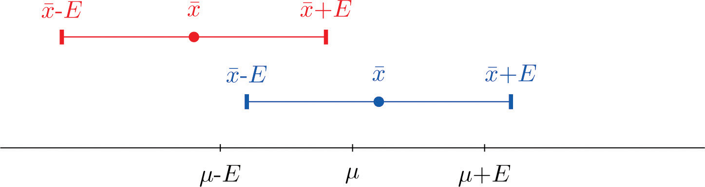
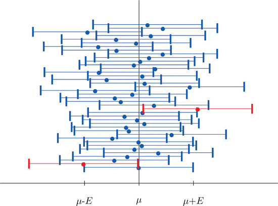
Figure \(\PageIndex{2}\) shows the intervals generated by a computer simulation of drawing \(40\) samples from a normally distributed population and constructing the \(95\%\) confidence interval for each one. We expect that about \( (0.05)(40)=2\) of the intervals so constructed would fail to contain the population mean \(\mu \), and in this simulation two of the intervals, shown in red, do.
It is standard practice to identify the level of confidence in terms of the area \(α\) in the two tails of the distribution of \(\overline{X}\) when the middle part specified by the level of confidence is taken out. This is shown in Figure \(\PageIndex{3}\), drawn for the general situation, and in Figure \(\PageIndex{4}\), drawn for \(95\%\) confidence.
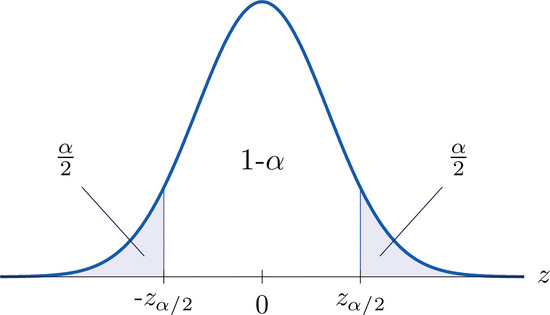
Remember from Section 5.4 that the \(z\)-value that cuts off a right tail of area \(c\) is denoted \(z_c\). Thus the number \(1.960\) in the example is \( z_{.025}\), which is \(z_{\frac{\alpha }{2}}\) for \(\alpha =1-0.95=0.05\).

For \(95\%\) confidence the area in each tail is \(\alpha /2=0.025\).
The level of confidence can be any number between \(0\) and \(100\%\), but the most common values are probably \(90\%\) \((\alpha =0.10)\), \(95\%\) \((\alpha =0.05)\), and \(99\%\) \((\alpha =0.01)\).
Thus in general for a \(100(1-\alpha )\%\) confidence interval, \(E=z_{\alpha /2}(\sigma /\sqrt{n})\), so the formula for the confidence interval is \(\bar{x}\pm z_{\alpha /2}(\sigma /\sqrt{n})\). While sometimes the population standard deviation \(\sigma\) is known, typically it is not. If not, for \(n\geq 30\) it is generally safe to approximate \(\sigma\) by the sample standard deviation \(s\).
- If \(\sigma\) is known: \[\bar{x}\pm z_{\alpha /2}\left ( \dfrac{\sigma }{\sqrt{n}} \right ) \nonumber \]
- If \(\sigma\) is unknown: \[\bar{x}\pm z_{\alpha /2}\left ( \dfrac{s}{\sqrt{n}} \right ) \nonumber \]
A sample is considered large when \(n\geq 30\).
As mentioned earlier, the number
\[E=z_{\alpha /2}\left ( \frac{\sigma }{\sqrt{n}} \right ) \nonumber \]
or
\[E=z_{\alpha /2}\left ( \frac{s}{\sqrt{n}} \right ) \nonumber \]
is called the margin of error of the estimate.
Find the number \(z_{\alpha /2}\) needed in construction of a confidence interval:
- when the level of confidence is \(90\%\);
- when the level of confidence is \(99\%\).
using the tables in Figure \(\PageIndex{5}\) below.
Solution:
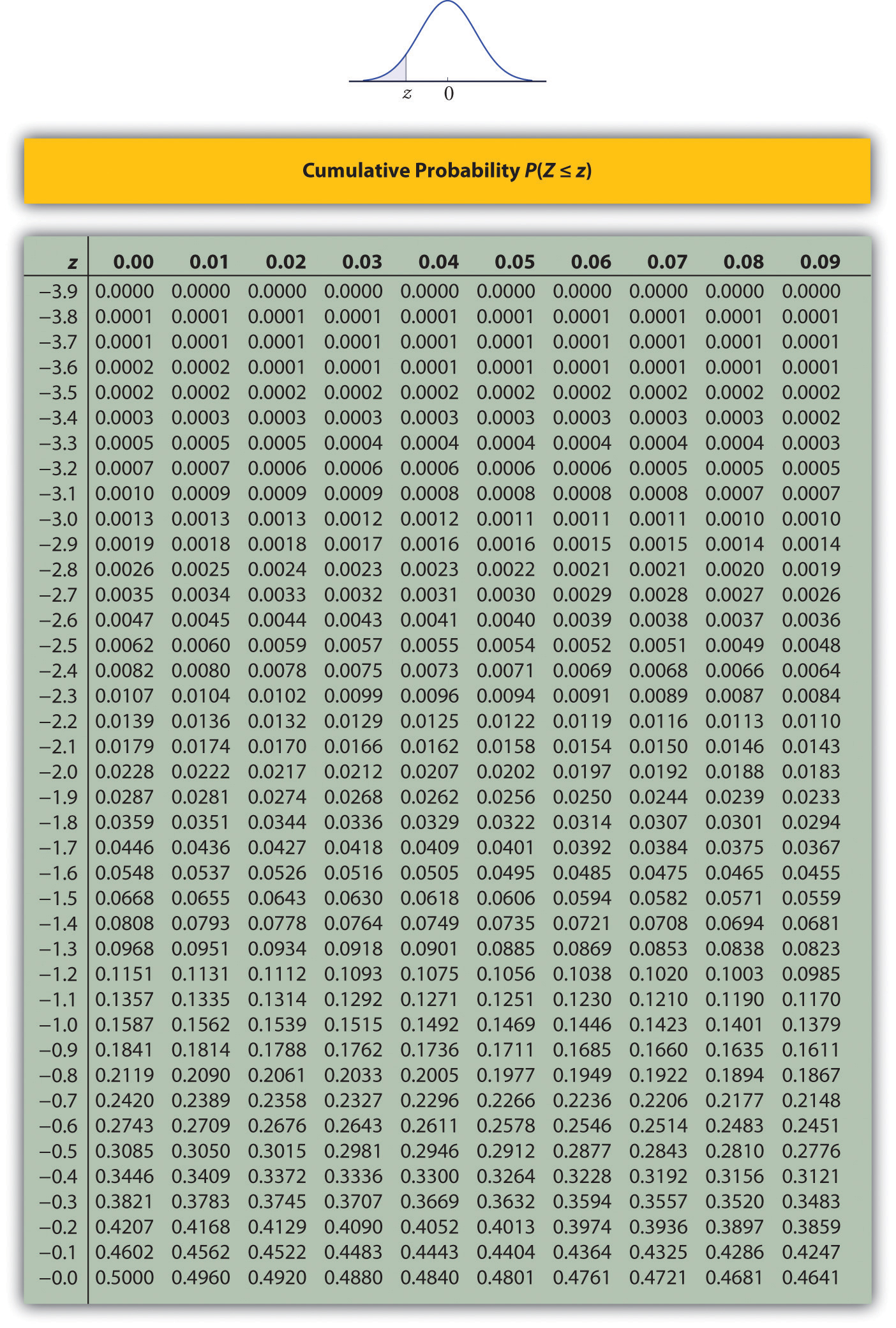
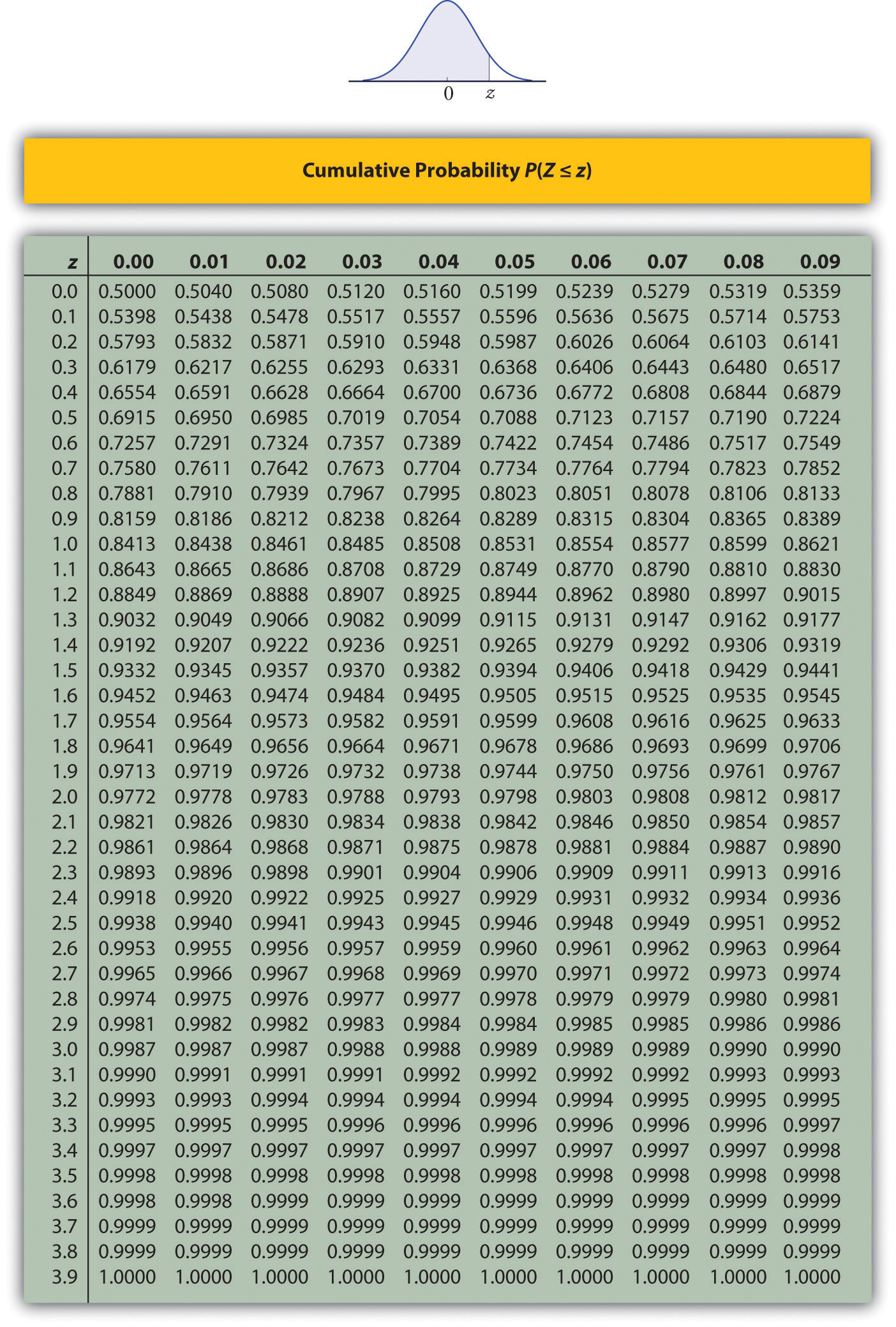
- For confidence level \(90\%\), \(\alpha =1-0.90=0.10\), so \(z_{\alpha /2}=z_{0.05}\). Since the area under the standard normal curve to the right of \(z_{0.05}\) is \(0.05\), the area to the left of \(z_{0.05}\) is \(0.95\). We search for the area \(0.9500\) in Figure \(\PageIndex{5}\). The closest entries in the table are \(0.9495\) and \(0.9505\), corresponding to \(z\)-values \(1.64\) and \(1.65\). Since \(0.95\) is halfway between \(0.9495\) and \(0.9505\) we use the average \(1.645\) of the \(z\)-values for \(z_{0.05}\).
- For confidence level \(99\%\), \(\alpha =1-0.99=0.01\), so \(z_{\alpha /2}=z_{0.005}\). Since the area under the standard normal curve to the right of \(z_{0.005}\) is \(0.005\), the area to the left of \(z_{0.005}\) is \(0.9950\). We search for the area \(0.9950\) in Figure \(\PageIndex{5}\). The closest entries in the table are \(0.9949\) and \(0.9951\), corresponding to \(z\)-values \(2.57\) and \(2.58\). Since \(0.995\) is halfway between \(0.9949\) and \(0.9951\) we use the average \(2.575\) of the \(z\)-values for \(z_{0.005}\).
Use Figure \(\PageIndex{6}\) below to find the number \(z_{\alpha /2}\) needed in construction of a confidence interval:
- when the level of confidence is \(90\%\);
- when the level of confidence is \(99\%\).
Solution:
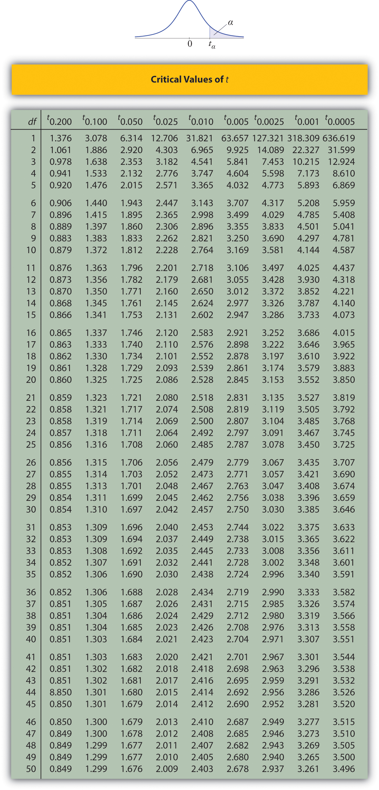
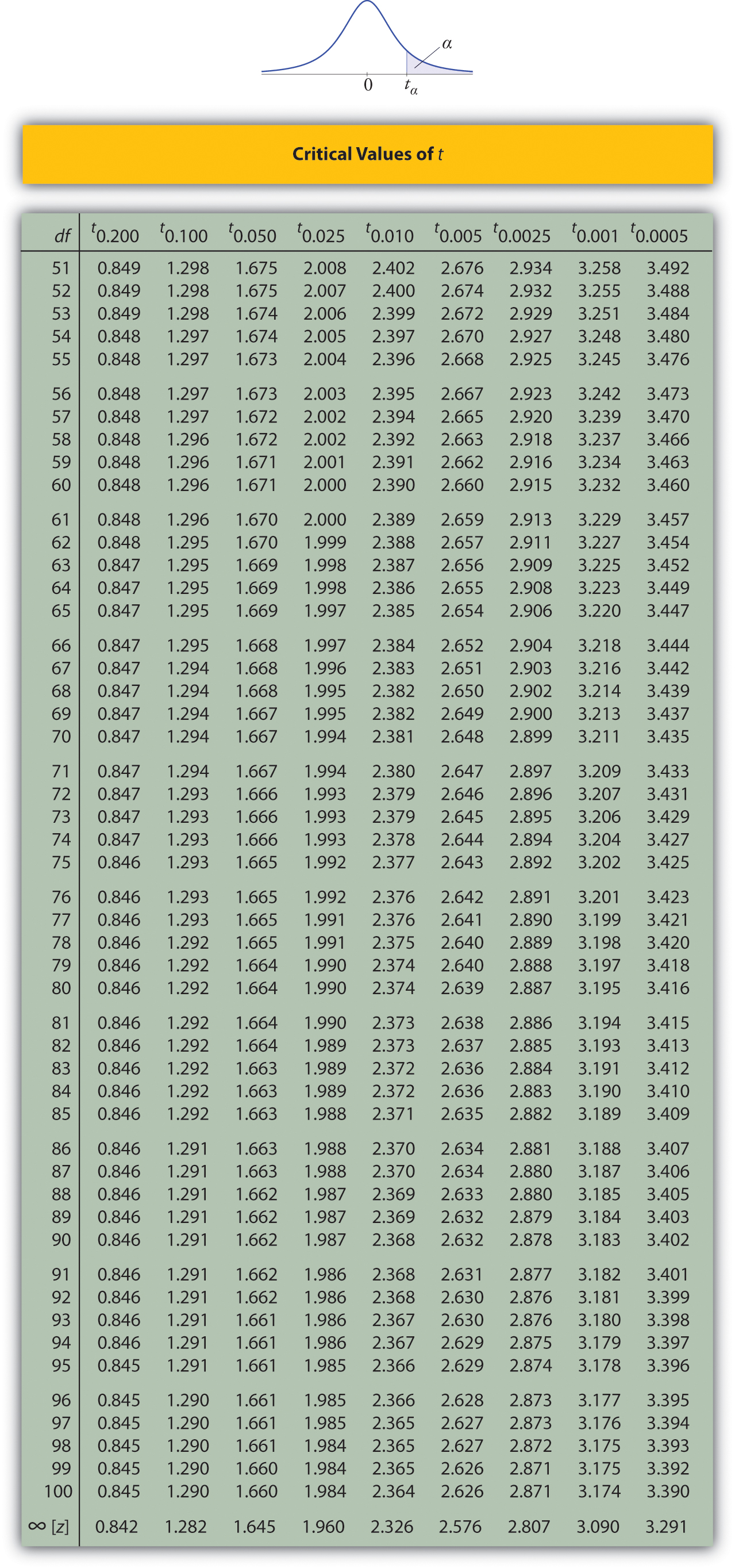
- In the next section we will learn about a continuous random variable that has a probability distribution called the Student \(t\)-distribution. Figure \(\PageIndex{6}\) gives the value \(t_c\) that cuts off a right tail of area \(c\) for different values of \(c\). The last line of that table, the one whose heading is the symbol \(\infty\) for infinity and \([z]\), gives the corresponding \(z\)-value \(z_c\) that cuts off a right tail of the same area \(c\). In particular, \(z_{0.05}\) is the number in that row and in the column with the heading \(t_{0.05}\). We read off directly that \(z_{0.05}=1.645\).
- In Figure \(\PageIndex{6}\) \(z_{0.005}\) is the number in the last row and in the column headed \(t_{0.005}\), namely \(2.576\).
Figure \(\PageIndex{6}\) can be used to find \(z_c\) only for those values of \(c\) for which there is a column with the heading \(t_c\) appearing in the table; otherwise we must use Figure \(\PageIndex{5}\) in reverse. But when it can be done it is both faster and more accurate to use the last line of Figure \(\PageIndex{6}\) to find \(z_c\) than it is to do so using Figure \(\PageIndex{5}\) in reverse.
A sample of size \(49\) has sample mean \(35\) and sample standard deviation \(14\). Construct a \(98\%\) confidence interval for the population mean using this information. Interpret its meaning.
Solution:
For confidence level \(98\%\), \(\alpha =1-0.98=0.02\), so \(z_{\alpha /2}=z_{0.01}\). From Figure \(\PageIndex{6}\) we read directly that \(z_{0.01}=2.326\).Thus
\[\bar{x}\pm z_{\alpha /2}\frac{s}{\sqrt{n}}=35\pm 2.326\left ( \frac{14}{\sqrt{49}} \right )=35\pm 4.652\approx 35\pm 4.7 \nonumber \]
We are \(98\%\) confident that the population mean \(\mu\) lies in the interval \([30.3,39.7]\), in the sense that in repeated sampling \(98\%\) of all intervals constructed from the sample data in this manner will contain \(\mu\).
A random sample of \(120\) students from a large university yields mean GPA \(2.71\) with sample standard deviation \(0.51\). Construct a \(90\%\) confidence interval for the mean GPA of all students at the university.
Solution:
For confidence level \(90\%\), \(\alpha =1-0.90=0.10\), so \(z_{\alpha /2}=z_{0.05}\). From Figure \(\PageIndex{6}\) we read directly that \(z_{0.05}=1.645\). Since \(n=120\), \(\bar{x}=2.71\), and \(s=0.51\),
\[\bar{x}\pm z_{\alpha /2}\frac{s}{\sqrt{n}}=2.71\pm 1.645\left ( \frac{0.51}{\sqrt{120}} \right )=2.71\pm 0.0766 \nonumber \]
One may be \(90\%\) confident that the true average GPA of all students at the university is contained in the interval \((2.71-0.08,2.71+0.08)=(2.63,2.79)\).
Key Takeaway
- A confidence interval for a population mean is an estimate of the population mean together with an indication of reliability.
- There are different formulas for a confidence interval based on the sample size and whether or not the population standard deviation is known.
- The confidence intervals are constructed entirely from the sample data (or sample data and the population standard deviation, when it is known).