In this section, we will go over how to round decimals to the nearest whole number, nearest tenth, nearest hundredth, etc. In most statistics applications that you will encounter, the numbers will not come out evenly, and you will need to round the decimal. We will also look at how to read scientific notation. A very common error that statistics students make is not noticing that the calculator is giving an answer in scientific notation.
For example, suppose that you used a calculator to find the probability that a randomly selected day in July will have a high temperature of over 90 degrees. Your calculator gives the answer: 0.4987230156. This is far too many digits for practical use, so it makes sense to round to just a few digits. By the end of this section you will be able to perform the rounding that is necessary to make unmanageable numbers manageable.
Brief Review of Decimal Language
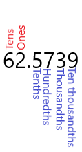
Consider the decimal number: 62.5739. There is a defined way to refer to each of the digits.
- The digit 6 is in the "Tens Place"
- The digit 2 is in the "Ones Place"
- The digit 5 is in the "Tenths Place"
- The digit 7 is in the "Hundredths Place"
- The digit 3 is in the "Thousandths Place"
- The digit 9 is in the "Ten-thousandths Place"
- We also say that 62 is the "Whole Number" part.

Keeping this example in mind will help you when you are asked to round to a specific place value.
Example \(\PageIndex{1}\)
It is reported that the mean number of classes that college students take each semester is 3.2541. Then the digit in the hundredths place is 5.
Rules of Rounding
Now that we have reviewed place values of numbers, we are ready to go over the process of rounding to a specified place value. When asked to round to a specified place value, the answer will erase all the digits after the specified digit. The process to deal with the other digits is best shown by examples.
Example \(\PageIndex{2}\): Case 1 - The Test Digit is Less Than 5
Round 3.741 to the nearest tenth.
Solution

Since the test digit (4) is less than 5, we just erase everything to the right of the tenths digit, 7. The answer is: 3.7.
Example \(\PageIndex{3}\): Case 2 - The Test Digit is 5 or Greater
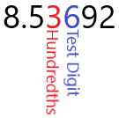
Round 8.53792 to the nearest hundredth.
Solution

Since the test digit (6) is 5 or greater, we add one to the hundredths digit and erase everything to the right of the hundredths digit, 3. Thus the 3 becomes a 4. The answer is: 8.54.
Example \(\PageIndex{4}\): Case 3 - The Test Digit is 5 or Greater and the rounding position digit is a 9
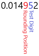
Round 0.014952 to four decimal places.
Solution

The test digit is 5, so we must round up. The rounding position is a 9 and adding 1 gives 10, which is not a single digit number. Instead look at the two digits to the left of the test digit: 49. If we add 1 to 49, we get 50. Thus the answer is 0.0150.
Applications
Rounding is used in most areas of statistics, since the calculator or computer will produce numerical answers with far more digits than are useful. If you are not told how many decimal places to round to, then you often want to think about the smallest number of decimals to keep so that no important information is lost. For example suppose you conducted a sample to find the proportion of college students who receive financial aid and the calculator presented 0.568429314. You could turn this into a percent at 56.8429314%. There are no applications where keeping this many decimal places is useful. If, for example, you wanted to present this finding to the student government, you might want to round to the nearest whole number. In this case the ones digit is 6 and the test digit is 8. Since 8 > 5, you add 1 to the ones digit. You can tell the student government that 57% of all college students receive financial aid.
Example \(\PageIndex{5}\)
Suppose that you found out that the probability that a randomly selected person with who has misused prescription opioids will transition to heroin is 0.04998713. Round this number to four decimal places.
Solution
The first four decimal places are 0.0499 and the test digit is 8. Since 8 > 5, we would like to add 1 to the fourth digit. Since this is a 9, we go to the next digit to the left. This is also a 9, so we go to the next one which is a 4. We can think of adding 0499 + 1 = 0500. Thus the answer is 0.0500. Note that we keep the last two 0's after the 5 to emphasize that this is accurate to the fourth decimal place.
Rounding and Arithmetic
Many times, we have to do arithmetic on numbers with several decimal places and want the answer rounded to a smaller number of decimal places. One question you might ask is should you round before you perform the arithmetic or after. For the most accurate result, you should always round after you preform the arithmetic if possible.
When asked to do arithmetic and present you answer rounded to a fixed number of decimal places, only round after performing the arithmetic.
Example \(\PageIndex{6}\)
Suppose you pick three cards from a 52 card deck with replacement and want to find the probability of the event, A, that none of the three cards will be a 2 through 7 of hearts. This probability is:
\[P\left(A\right)=\left(0.8846\right)^3 \nonumber\]
Round the answer to 2 decimal places.
Solution
Note that we have to first perform the arithmetic. With a computer or calculator we get:
\[0.8846^3=\text{0.69221467973} \nonumber\]
Now we round to two decimal places. Notice that the hundredths digit is a 9 and the test digit is a 2. Thus the 9 remains unchanged and everything to the right of the 9 goes away. the result is
\[P\left(A\right)\approx0.69 \nonumber\]
If we mistakenly rounded 0.8846 to two decimal places (0.88) and then cubed the answer we would have gotten 0.68 which is not the correct answer.
Scientific Notation
When a calculator presents a number in scientific notation, we must pay attention to what this represents. The standard way of writing a number in scientific notation is writing the number as a product of a number greater than or equal 1 but less than 10 followed by a power of 10. For example:
\[ 602,000,000,000,000,000,000,000 = 6.02 \times 10^{23} \nonumber\]
The main purpose of scientific notation is to allow us to write very large numbers or numbers very close to 0 without having to use so many digits. Most calculators and computers use a different notation for scientific notation, most likely because the superscript is difficult to render on a screen. For example, with a calculator:
\[0.00000032 = 3.2E-7 \nonumber\]
Notice that to arrive at 3.2, the decimal needed to be moved 7 places to the right.
Example \(\PageIndex{7}\)
A calculator displays:
\[2.0541E6 \nonumber\]
Write this number in decimal form.
Solution
Notice that the number following E is 6. This means move the decimal over 6 places to the right. The first 4 moves is natural, but for the last 2 moves, there are no numbers to move the decimal place past. We can always add extra zeros after the last number to the right of the decimal place:
\[2.0541E6 = 2.054100E6 \nonumber\]
Now we can move the decimal place to the right 6 places to get
\[2.0541E6 = 2.054100E6 = 2,054,100 \nonumber \]
Example \(\PageIndex{8}\)
If you use a calculator or computer to find the probability of flipping a coin 27 times and getting all heads, then it will display:
\[ 7.45E−9 \nonumber\]
Write this number in decimal form.
Solution
Many students will forget to look for the "E" and just write that the probability is 7.45, but probabilities can never be bigger than 1. You can not have a 745% chance of it occurring. Notice that the number following E is −9. Since the power is negative, this means move the decimal to the left, and in particular 9 places to the left. There is only one digit to the left of the decimal place, so we need to insert 8 zeros:
\[ 7.45E−9 = 000000007.45E−9 \nonumber\]
Now we can move the decimal place to the right 9 places to the left to get
\[ 7.45E−9 = 000000007.45E−9 = 0.00000000745 \nonumber\]


