7.4: Steps of the Hypothesis Testing Process

A Four-Step Procedure

The process of testing hypotheses follows a simple four-step procedure. This process will be what we use for the remainder of the textbook and course, and although the hypothesis and statistics we use will change, this process will not.

Step 1: State the Hypotheses

Your hypotheses are the first thing you need to lay out. Otherwise, there is nothing to test! You have to state the null hypothesis (which is what we test) and the alternative hypothesis (which is what we expect). These should be stated mathematically as they were presented above and in words, explaining in normal English what each one means in terms of the research question.

Step 2: Find the Critical Values

Next, we formally lay out the criteria we will use to test our hypotheses. There are two pieces of information that inform our critical values: \(\alpha\), which determines how much of the area under the curve composes our rejection region, and the directionality of the test, which determines where the region will be.

Step 3: Calculate the Test Statistic and Effect Size

Once we have our hypotheses and the standards we use to test them, we can collect data and calculate our test statistic—in this case, z. This step is where the vast majority of differences in future chapters will arise: different tests used for different data are calculated in different ways, but the way we use and interpret them remains the same. As part of this step, we will also calculate the effect size to better quantify the magnitude of the difference between our groups. Although effect size is not considered part of hypothesis testing, reporting it as part of the results is an approved convention.

Step 4: Make the Decision

Finally, once we have obtained our test statistic, we can compare it to our critical value and decide whether we should reject or fail to reject the null hypothesis. When we do this, we must interpret the decision in relation to our research question, stating what we concluded, what we based our conclusion on, and the specific statistics we obtained.

Example A: Movie Popcorn

Let’s see how hypothesis testing works in action by working through an example. Say that a movie theater owner likes to keep a very close eye on how much popcorn goes into each bag sold, so he knows that the average bag has 8 cups of popcorn and that this varies a little bit, about half a cup. That is, the known population mean is \(\mu=8.00\) and the known population standard deviation is \(\sigma = 0.50\). The owner wants to make sure that the newest employee is filling bags correctly, so over the course of a week, he randomly assesses 25 bags filled by the employee to test for a difference (N = 25). He doesn’t want bags over-filled or under-filled, so he looks for differences in both directions. This scenario has all of the information we need to begin our hypothesis testing procedure.

Step 1: State the Hypotheses

Our manager is looking for a difference in the mean weight of popcorn bags compared to the population mean of 8. We will need both a null and an alternative hypothesis written both mathematically and in words. We’ll always start with the null hypothesis:

\[
\begin{aligned}
H_0: &\ \text{There is no difference in the weight of popcorn bags from this employee} \\
H_0: &\ \mu = 8.00 \nonumber
\end{aligned}
\]

Notice that we phrase the hypothesis in terms of the population parameter \(\mu\), which in this case would be the true average weight of bags filled by the new employee. Our assumption of no difference, the null hypothesis, is that this mean is exactly the same as the known population mean value we want it to match, 8.00. Now let’s do the alternative:

\[
\begin{aligned}
H_A: &\ \text{There is a difference in the weight of popcorn bags from this employee} \\
H_A: &\ \mu \neq 8.00 \nonumber
\end{aligned}
\]

In this case, we don’t know if the bags will be too full or not full enough, so we do a two-tailed alternative hypothesis that there is a difference.

Step 2: Find the Critical Values

Our critical values are based on two things: the directionality of the test and the level of significance. We decided in Step 1 that a two-tailed test is the appropriate directionality. We were given no information about the level of significance, so we assume that \(\alpha = .05 \) is what we will use. As stated earlier in the chapter, the critical values for a two-tailed z test at \(\alpha = .05 \) are z* = ±1.96. This will be the criterion we use to test our hypothesis. We can now draw out our distribution, as shown in Figure \(\PageIndex{1}\), so we can visualize the rejection region and make sure it makes sense.

Figure \(\PageIndex{1}\): Rejection region for z* = ±1.96. (“Rejection Region z = +-1.96” by Judy Schmitt is licensed under CC BY-NC-SA 4.0.)

Step 3: Calculate the Test Statistic and Effect Size

Now we come to our formal calculations. Let’s say that the manager collects data and finds that the average weight of this employee’s popcorn bags is M = 7.75 cups. We can now plug this value, along with the values presented in the original problem, into our equation for z:

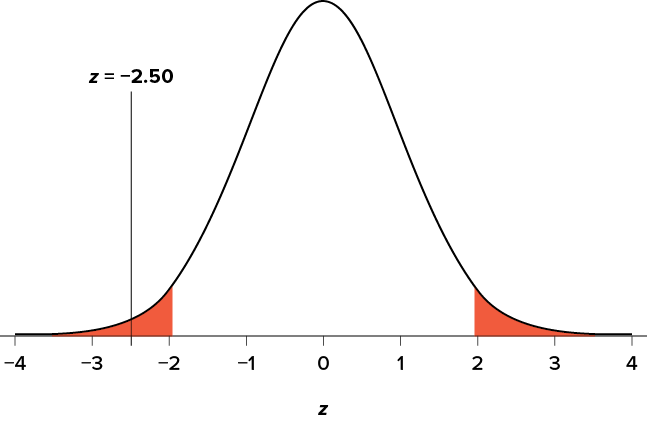
\[z = \frac{7.75-8.00}{0.50/\sqrt{25}} = \frac{-0.25}{0.10} = -2.50 \nonumber \]

So our test statistic is z = −2.50, which we can draw onto our rejection region distribution as shown in Figure \(\PageIndex{2}\).

Figure \(\PageIndex{2}\): Test statistic location. (“Test Statistic Location z = -2.50” by Judy Schmitt is licensed under CC BY-NC-SA 4.0.

Effect Size

When we reject the null hypothesis, we are stating that the difference we found was statistically significant, but we have mentioned several times that this tells us nothing about practical significance. To get an idea of the actual size of what we found, we can compute a new statistic called an effect size. Effect size gives us an idea of how large, important, or meaningful a statistically significant effect is. For mean differences like we calculated here, our effect size is Cohen’s d:

\[d = \frac{M-\mu}{\sigma} \nonumber \]

This is very similar to our formula for z, but we no longer take into account the sample size (since overly large samples can make it too easy to reject the null). Cohen’s d is interpreted in units of standard deviations, just like z. For our example:

\[d = \frac{7.75-8.00}{0.50} = \frac{-0.25}{0.50} = 0.50 \nonumber \]

Cohen’s d is interpreted as small, moderate, or large. Specifically, d = 0.20 is small, d = 0.50 is moderate, and d = 0.80 is large. Obviously, values can fall in between these guidelines, so we should use our best judgment and the context of the problem to make our final interpretation of size. Our effect size happens to be exactly equal to one of these, so we say that there is a moderate effect.

Effect sizes are incredibly useful and provide important information and clarification that overcomes some of the weaknesses of hypothesis testing. Any time you perform a hypothesis test, whether statistically significant or not, you should always calculate and report the effect size.

Step 4: Make the Decision

Looking at Figure \(\PageIndex{2}\), we can see that our obtained z statistic falls in the rejection region. We can also directly compare it to our critical value: in terms of absolute value, −2.50 > −1.96, so we reject the null hypothesis. We can now write our conclusion:

Reject H0. Based on the sample of 25 bags, we can conclude that the average popcorn bag from this employee is smaller (M = 7.75 cups) than the average weight of popcorn bags at this movie theater, and the effect size was moderate, z = −2.50, p < .05, d = 0.50.

When we write our conclusion, we write out the words to communicate what it actually means, but we also include the average sample size we calculated (the exact location doesn’t matter, just somewhere that flows naturally and makes sense), the z statistic and p value, and the effect size. We don’t know the exact p-value, but we do know that because we rejected the null, it must be less than \(\alpha\).

Example B: Office Temperature

Let’s do another example to solidify our understanding. Let’s say that the office building you work in is supposed to be kept at 74 degrees Fahrenheit during the summer months, but is allowed to vary by 1 degree in either direction. You suspect that, as a cost-saving measure, the temperature was secretly set higher. You set up a formal way to test your hypothesis.

Step 1: State the Hypotheses

You start by laying out the null hypothesis:

\[
\begin{aligned}
H_0: &\ \text{There is no difference in the average building temperature} \\
H_0: &\ \mu = 74 \nonumber
\end{aligned}
\]

Next, you state the alternative hypothesis. You have reason to suspect a specific direction of change, so you make a one-tailed test:

\[
\begin{aligned}
H_A: &\ \text{The average building temperature is higher than claimed} \\
H_A: &\ \mu > 74 \nonumber
\end{aligned}
\]

Step 2: Find the Critical Values

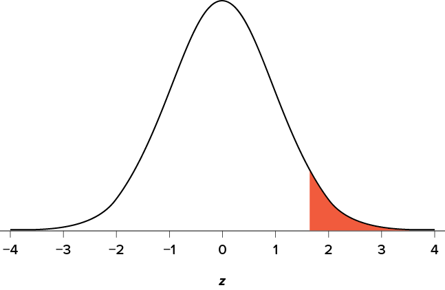
You know that the most common level of significance is \(\alpha=.05\), so you keep that the same and know that the critical value for a one-tailed z test is z* = 1.645. To keep track of the directionality of the test and rejection region, you draw out your distribution as shown in Figure \(\PageIndex{3}\).

Figure \(\PageIndex{3}\): Rejection region. (“Rejection Region z = 1.645” by Judy Schmitt is licensed under CC BY-NC-SA 4.0.)

Step 3: Calculate the Test Statistic and Effect Size

Now that you have everything set up, you spend one week collecting temperature data:

• Monday: 77°
• Tuesday: 76°
• Wednesday: 74°
• Thursday: 78°
• Friday: 78°

You calculate the average of these scores to be M = 76.6 degrees. You use this to calculate the test statistic, using \(\mu=74\) (the supposed average temperature), \(\sigma=1.00\) (how much the temperature should vary), and n = 5 (how many data points you collected):

\[z = \frac{76.60-74.00}{1.00/\sqrt{5}} = \frac{2.60}{0.45} = 5.78 \nonumber \]

This value falls so far into the tail that it cannot even be plotted on the distribution (Figure \(\PageIndex{4}\))! Because the result is significant, you also calculate an effect size:

\[d = \frac{76.60-74.00}{1.00} = \frac{2.60}{1.00} = 2.60 \nonumber \]

The effect size you calculate is definitely large, meaning someone has some explaining to do!

Figure \(\PageIndex{4}\): Obtained z statistic. (“Obtained z = 5.77” by Judy Schmitt is licensed under CC BY-NC-SA 4.0.)

Step 4: Make the Decision

You compare your obtained z statistic, z = 5.77, to the critical value, z* = 1.645, and find that z > z*. Therefore, you reject the null hypothesis, concluding:

Reject \(H_0\). Based on 5 observations, the average temperature (M = 76.6 degrees) is statistically significantly higher than it is supposed to be, and the effect size was large, z = 5.77, p < .05, d = 2.60.

Example C: Different Significance Level

Finally, let’s take a look at an example phrased in generic terms, rather than in the context of a specific research question, to see the individual pieces one more time. This time, however, we will use a stricter significance level, \(\alpha=.05\), to test the hypothesis.

Step 1: State the Hypotheses

We will use 60 as an arbitrary null hypothesis value:

\[
\begin{aligned}
H_0: &\ \text{The average score does not differ from the population} \\
H_0: &\ \mu = 60 \nonumber
\end{aligned}
\]

We will assume a two-tailed test:

\[
\begin{aligned}
H_A: &\ \text{The average score does differ} \\
H_A: &\ \mu \neq 60 \nonumber
\end{aligned}
\]

Step 2: Find the Critical Values

We have seen the critical values for z tests at \(\alpha=.05\) levels of significance several times. To find the values for \(\alpha=.01\), we will go to the Standard Normal Distribution Table and find the z score cutting off .005 (.01 divided by 2 for a two-tailed test) of the area in the tail, which is z* = ±2.575. Notice that this cutoff is much higher than it was for \(\alpha=.05\). This is because we need much less of the area in the tail, so we need to go very far out to find the cutoff. As a result, this will require a much larger effect or a much larger sample size in order to reject the null hypothesis.

Step 3: Calculate the Test Statistic and Effect Size

We can now calculate our test statistic. We will use \(\sigma=10\) as our known population standard deviation and the following data to calculate our sample mean from the following dataset:

Dataset \(\PageIndex{1}\)

61, 65, 58, 54, 60, 62, 61, 59, 61, 63

The average of these scores is M = 60.40. From this, we calculate our z statistic as:

\[z = \frac{60.40-60.00}{10.00/\sqrt{10}} = \frac{0.40}{3.16} = 0.13 \nonumber \]

The Cohen’s d effect size calculation is:

\[d = \frac{M-\mu}{\sigma} = \frac{60.40-60.00}{10.00} = \frac{0.40}{10.00} = 0.04 \nonumber \]

Step 4: Make the Decision

Our obtained z statistic, z = 0.13, is very small. It is much less than our critical value of 2.575. Thus, this time, we fail to reject the null hypothesis. Our conclusion would look something like:

Fail to reject \(H_0\). Based on the sample of 10 scores, we cannot conclude that there is an effect causing the mean (M = 60.40) to be statistically significantly different from 60.00, z = 0.13, p > .01, d = 0.04, and the effect size supports this interpretation.

Notice two things about the end of the conclusion. First, we wrote that p is greater than instead of p is less than, like we did in the previous two examples. This is because we failed to reject the null hypothesis. We don’t know exactly what the p-value is, but we know it must be larger than the \(\alpha\) level we used to test our hypothesis. Second, we used .01 instead of the usual .05, because this time we tested at a different level. The number you compare to the p-value should always be the significance level you test at.

Video: Hypothesis testing and p-values

Hypothesis testing and p-values on YouTube.

Test Your Knowledge

Question \(\PageIndex{1}\)

Question \(\PageIndex{2}\)

Question \(\PageIndex{3}\)