7.4: Using the Central Limit Theorem
- Last updated
- Save as PDF
- Page ID
- 15505
It is important for you to understand when to use the central limit theorem (clt). If you are being asked to find the probability of the mean, use the clt for the mean. If you are being asked to find the probability of a sum or total, use the clt for sums. This also applies to percentiles for means and sums.
If you are being asked to find the probability of an individual value, do not use the clt. Use the distribution of its random variable.
Law of Large Numbers
The law of large numbers says that if you take samples of larger and larger size from any population, then the mean \(\bar{x}\) of the sample tends to get closer and closer to \(\mu\). From the central limit theorem, we know that as \(n\) gets larger and larger, the sample means follow a normal distribution. The larger \(n\) gets, the smaller the standard deviation gets. (Remember that the standard deviation for \(\bar{X}\) is \(\dfrac{\sigma}{\sqrt{n}}\).) This means that the sample mean \(\bar{x}\) must be close to the population mean \(\mu\). We can say that \(\mu\) is the value that the sample means approach as \(n\) gets larger. The central limit theorem illustrates the law of large numbers.
Example \(\PageIndex{1}\)
A study involving stress is conducted among the students on a college campus. The stress scores follow a uniform distribution with the lowest stress score equal to one and the highest equal to five. Using a sample of 75 students, find:
- The probability that the mean stress score for the 75 students is less than two.
- The 90th percentile for the mean stress score for the 75 students.
- The probability that the total of the 75 stress scores is less than 200.
- The 90th percentile for the total stress score for the 75 students.
Solutions
Let \(X =\) one stress score.
Problems a and b ask you to find a probability or a percentile for a mean. Problems c and d ask you to find a probability or a percentile for a total or sum. The sample size, \(n\), is equal to 75.
Since the individual stress scores follow a uniform distribution, \(X \sim U(1, 5)\) where \(a = 1\) and \(b = 5\).
\[\mu_{x} = \dfrac{a+b}{2} = \dfrac{1+5}{2} = 3\]
\[\sigma_{x} = \sqrt{\dfrac{(b-a)^{2}}{12}} = \sqrt{\dfrac{(5-1)^{2}}{12}} = 1.15\]
For problems 1. and 2., let \(\bar{X} =\) the mean stress score for the 75 students. Then,
\[\bar{X} \sim N\left(3, \dfrac{1,15}{\sqrt{75}}\right)\]
where \(n = 75\).
- Find \(P(\bar{x} < 2)\). Draw the graph.
- Find the 90th percentile for the mean of 75 stress scores. Draw a graph.
- Find \(P(\sum x < 2000)\). Draw the graph.
- Find the 90th percentile for the total of 75 stress scores. Draw a graph.
Answers
a. \(P(\bar{x} < 2) = 0\)
The probability that the mean stress score is less than two is about zero.
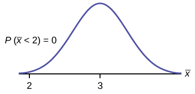
normalcdf \(\left(1,2,3,\dfrac{1.15}{\sqrt{75}}\right) = 0\)
REMINDER
The smallest stress score is one
b. Let \(k =\) the 90th percentile.
Find \(k\), where \(P(\bar{x} < k) = 0.90\).
\(k = 3.2\)
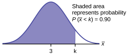
The 90th percentile for the mean of 75 scores is about 3.2. This tells us that 90% of all the means of 75 stress scores are at most 3.2, and that 10% are at least 3.2.
invNorm\(\left(0.90,3,1.\dfrac{1.15}{\sqrt{75}}\right) = 3.2\)
For problems c and d, let \(\sum X =\) the sum of the 75 stress scores. Then,
\[\sum X \sim N((75)(3), (\sqrt{75})(1.15))\]
c. The mean of the sum of 75 stress scores is \((75)(3) = 225\)
The standard deviation of the sum of 75 stress scores is \((\sqrt{75})(1.15) = 9.96\)
\(P(\sum x < 200)\)
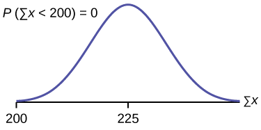
The probability that the total of 75 scores is less than 200 is about zero.
normalcdf \(75,200,(75)(3),(\sqrt{75})(1.15)\).
REMINDER
The smallest total of 75 stress scores is 75, because the smallest single score is one.
d. Let \(k =\) the 90th percentile.
Find \(k\) where \(P(\sum x < k) = 0.90\).
\(k = 237.8\)
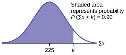
The 90th percentile for the sum of 75 scores is about 237.8. This tells us that 90% of all the sums of 75 scores are no more than 237.8 and 10% are no less than 237.8.
invNorm\(\left(0.90, (75)(3), (\sqrt{75})(1.15)\right) = 237.8\)
Exercise \(\PageIndex{1}\)
Use the information in Example \(\PageIndex{1}\), but use a sample size of 55 to answer the following questions.
- Find \(P(\bar{x} < 7)\).
- Find \(P(\sum x < 7)\).
- Find the 80th percentile for the mean of 55 scores.
- Find the 85th percentile for the sum of 55 scores.
Answer
- 0.0265
- 0.2789
- 3.13
- 173.84
Example \(\PageIndex{2}\)
Suppose that a market research analyst for a cell phone company conducts a study of their customers who exceed the time allowance included on their basic cell phone contract; the analyst finds that for those people who exceed the time included in their basic contract, the excess time used follows an exponential distribution with a mean of 22 minutes.
Consider a random sample of 80 customers who exceed the time allowance included in their basic cell phone contract.
Let \(X =\) the excess time used by one INDIVIDUAL cell phone customer who exceeds his contracted time allowance.
\(X \sim Exp\left(\dfrac{1}{22}\right)\). From previous chapters, we know that \(\mu = 22\) and \(\sigma = 22\).
Let \(\bar{X}\) = the mean excess time used by a sample of \(n = 80\) customers who exceed their contracted time allowance.
\[\bar{X} \sim N\left(22,\dfrac{22}{\sqrt{80}}\right)\]
by the central limit theorem for sample means
- Find the probability that the mean excess time used by the 80 customers in the sample is longer than 20 minutes. This is asking us to find \(P(\bar{x} > 20)\). Draw the graph.
- Suppose that one customer who exceeds the time limit for his cell phone contract is randomly selected. Find the probability that this individual customer's excess time is longer than 20 minutes. This is asking us to find \(P(x > 20)\).
- Explain why the probabilities in parts a and b are different.
- Find the 95th percentile for the sample mean excess time for samples of 80 customers who exceed their basic contract time allowances. Draw a graph.
Answer
- Find: \(P(\bar{x} > 20)\)
\(P(\bar{x} > 20) = 0.79199\) using
normalcdf\(\left(20,1\text{E}99,22,\dfrac{22}{\sqrt{80}}\right)\)The probability is 0.7919 that the mean excess time used is more than 20 minutes, for a sample of 80 customers who exceed their contracted time allowance.
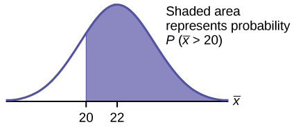
Figure \(\PageIndex{5}\).
REMINDER
1E99 = 1099 and –1E99 = –1099. Press the
EEkey for E. Or just use 1099 instead of 1E99. - Find \(P(x > 20)\). Remember to use the exponential distribution for an individual: \(X \sim Exp\left(\dfrac{1}{22}\right)\). \(P(x > 20) = e^{(−\left(\dfrac{1}{22}\right)(20))}\) or \(e^{(–0.04545(20))} = 0.4029\)
-
- \(P(x > 20) = 0.4029\) but \(P(\bar{x} > 20) = 0.7919\)
- The probabilities are not equal because we use different distributions to calculate the probability for individuals and for means.
- When asked to find the probability of an individual value, use the stated distribution of its random variable; do not use the clt. Use the clt with the normal distribution when you are being asked to find the probability for a mean.
- Let \(k\) = the 95th percentile. Find \(k\) where \(P(\bar{x} < k) = 0.95\)
\(k = 26.0\) using
invNorm\(\left(0.95,22,\dfrac{22}{\sqrt{80}}\right) = 26.0\)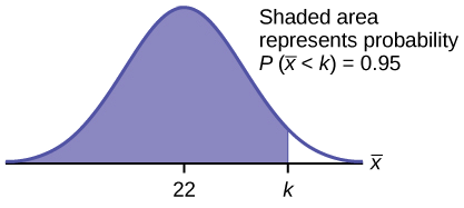
Figure \(\PageIndex{6}\).
The 95th percentile for the sample mean excess time used is about 26.0 minutes for random samples of 80 customers who exceed their contractual allowed time.
Ninety five percent of such samples would have means under 26 minutes; only five percent of such samples would have means above 26 minutes.
Exercise \(\PageIndex{2}\)
Use the information in Example \(\PageIndex{2}\), but change the sample size to 144.
- Find \(P(20 < \bar{x} < 30)\).
- Find \(P(\sum x \text{ is at least } 3,000)\).
- Find the 75th percentile for the sample mean excess time of 144 customers.
- Find the 85th percentile for the sum of 144 excess times used by customers.
Answer
- 0.8623
- 0.7377
- 23.2
- 3,441.6
Example \(\PageIndex{3}\)
In the United States, someone is sexually assaulted every two minutes, on average, according to a number of studies. Suppose the standard deviation is 0.5 minutes and the sample size is 100.
- Find the median, the first quartile, and the third quartile for the sample mean time of sexual assaults in the United States.
- Find the median, the first quartile, and the third quartile for the sum of sample times of sexual assaults in the United States.
- Find the probability that a sexual assault occurs on the average between 1.75 and 1.85 minutes.
- Find the value that is two standard deviations above the sample mean.
- Find the IQR for the sum of the sample times.
Answer
- We have, \(\mu_{x} = \mu = 2\) and \(\sigma_{x} = \dfrac{\sigma}{\sqrt{n}} = \dfrac{0.5}{10} = 0.05\). Therefore:
- 50th percentile \(= \mu_{x} = \mu = 2\)
- 25th percentile \(= \text{invNorm}(0.25,2,0.05) = 1.97\)
- 75th percentile \(= \text{invNorm}(0.75,2,0.05) = 2.03\)
- We have \(\mu_{\sum X} = n(\mu_{x}) = 100(2)\) and \(\sigma_{\mu X} = \sqrt{n}(\sigma_{x}) = 10(0.5) = 5\). Therefore
- 50th percentile = \(\mu_{\sum X} = n(\mu_{X}) = 100(2) = 200\)
- 25th percentile \(= \text{invNorm}(0.25,200,5) = 196.63\)
- 75th percentile \(= \text{invNorm}(0.75,200,5) = 203.37\)
- \(P(1.75 < bar{x} < 1.85) =\)
normalcdf\((1.75,1.85,2,0.05) = 0.0013\) - Using the \(z\)-score equation, \(z = \dfrac{\bar{x} - \mu_{\bar{x}}}{\sigma_{\bar{x}}}\), and solving for \(x\), we have \(x = 2(0.05) + 2 = 2.1\)
- The \(IQR\) is 75th percentile – 25th percentile \(= 203.37 – 196.63 = 6.74\)
Exercise \(\PageIndex{3}\)
Based on data from the National Health Survey, women between the ages of 18 and 24 have an average systolic blood pressures (in mm Hg) of 114.8 with a standard deviation of 13.1. Systolic blood pressure for women between the ages of 18 to 24 follow a normal distribution.
- If one woman from this population is randomly selected, find the probability that her systolic blood pressure is greater than 120.
- If 40 women from this population are randomly selected, find the probability that their mean systolic blood pressure is greater than 120.
- If the sample were four women between the ages of 18 to 24 and we did not know the original distribution, could the central limit theorem be used?
Answer
- \(P(x > 120)\) =
normalcdf\((120,99,114.8,13.1) = 0.0272\). There is about a 3%, that the randomly selected woman will have systolics blood pressure greater than 120. - \(P(\bar{x} > 120) =\)
normalcdf\(\left(120,114.8,\dfrac{13.1}{\sqrt{40}}\right) = 0.006\). There is only a 0.6% chance that the average systolic blood pressure for the randomly selected group is greater than 120. - The central limit theorem could not be used if the sample size were four and we did not know the original distribution was normal. The sample size would be too small.
Example \(\PageIndex{4}\)
A study was done about violence against prostitutes and the symptoms of the posttraumatic stress that they developed. The age range of the prostitutes was 14 to 61. The mean age was 30.9 years with a standard deviation of nine years.
- In a sample of 25 prostitutes, what is the probability that the mean age of the prostitutes is less than 35?
- Is it likely that the mean age of the sample group could be more than 50 years? Interpret the results.
- In a sample of 49 prostitutes, what is the probability that the sum of the ages is no less than 1,600?
- Is it likely that the sum of the ages of the 49 prostitutes is at most 1,595? Interpret the results.
- Find the 95th percentile for the sample mean age of 65 prostitutes. Interpret the results.
- Find the 90th percentile for the sum of the ages of 65 prostitutes. Interpret the results.
Answer
- \(P(\bar{x} < 35) =\)
normalcdf\((-E99,35,30.9,1.8) = 0.9886\) - \(P(\bar{x} > 50) =\)
normalcdf\((50, E99,30.9,1.8) \approx 0\). For this sample group, it is almost impossible for the group’s average age to be more than 50. However, it is still possible for an individual in this group to have an age greater than 50. - \(P(\sum x \geq 1,600) =\)
normalcdf\((1600,E99,1514.10,63) = 0.0864\) - \(P(\sum x \leq 1,595) =\)
normalcdf\((-E99,1595,1514.10,63) = 0.9005\). This means that there is a 90% chance that the sum of the ages for the sample group \(n = 49\) is at most 1595. - The 95th percentile =
invNorm\((0.95,30.9,1.1) = 32.7\). This indicates that 95% of the prostitutes in the sample of 65 are younger than 32.7 years, on average. - The 90th percentile =
invNorm\((0.90,2008.5,72.56) = 2101.5\). This indicates that 90% of the prostitutes in the sample of 65 have a sum of ages less than 2,101.5 years.
Exercise \(\PageIndex{4}\)
According to Boeing data, the 757 airliner carries 200 passengers and has doors with a mean height of 72 inches. Assume for a certain population of men we have a mean of 69.0 inches and a standard deviation of 2.8 inches.
- What mean doorway height would allow 95% of men to enter the aircraft without bending?
- Assume that half of the 200 passengers are men. What mean doorway height satisfies the condition that there is a 0.95 probability that this height is greater than the mean height of 100 men?
- For engineers designing the 757, which result is more relevant: the height from part a or part b? Why?
Answer
- We know that \(\mu_{x} = \mu = 69\) and we have \(\sigma_{x} = 2.8\). The height of the doorway is found to be
invNorm\((0.95,69,2.8) = 73.61\) - We know that \(\mu_{x} = \mu = 69\) and we have \(\sigma_{x} = 2.8\). So,
invNorm\((0.95,69,0.28) = 69.49\) - When designing the doorway heights, we need to incorporate as much variability as possible in order to accommodate as many passengers as possible. Therefore, we need to use the result based on part a.
Historical Note: Normal Approximation to the Binomial
Historically, being able to compute binomial probabilities was one of the most important applications of the central limit theorem. Binomial probabilities with a small value for \(n\)(say, 20) were displayed in a table in a book. To calculate the probabilities with large values of \(n\), you had to use the binomial formula, which could be very complicated. Using the normal approximation to the binomial distribution simplified the process. To compute the normal approximation to the binomial distribution, take a simple random sample from a population. You must meet the conditions for a binomial distribution:
- there are a certain number \(n\) of independent trials
- the outcomes of any trial are success or failure
- each trial has the same probability of a success \(p\)
Recall that if \(X\) is the binomial random variable, then \(X \sim B(n, p)\). The shape of the binomial distribution needs to be similar to the shape of the normal distribution. To ensure this, the quantities \(np\) and \(nq\) must both be greater than five (\(np > 5\) and \(nq > 5\)); the approximation is better if they are both greater than or equal to 10). Then the binomial can be approximated by the normal distribution with mean \(\mu = np\) and standard deviation \(\sigma = \sqrt{npq}\). Remember that \(q = 1 - p\). In order to get the best approximation, add 0.5 to \(x\) or subtract 0.5 from \(x\) (use \(x + 0.5\) or \(x - 0.5\)). The number 0.5 is called the continuity correction factor and is used in the following example.
Example \(\PageIndex{5}\)
Suppose in a local Kindergarten through 12th grade (K - 12) school district, 53 percent of the population favor a charter school for grades K through 5. A simple random sample of 300 is surveyed.
- Find the probability that at least 150 favor a charter school.
- Find the probability that at most 160 favor a charter school.
- Find the probability that more than 155 favor a charter school.
- Find the probability that fewer than 147 favor a charter school.
- Find the probability that exactly 175 favor a charter school.
Let \(X =\) the number that favor a charter school for grades K trough 5. \(X \sim B(n, p)\) where \(n = 300\) and \(p = 0.53\). Since \(np > 5\) and \(nq > 5\), use the normal approximation to the binomial. The formulas for the mean and standard deviation are \(\mu = np\) and \(\sigma = \sqrt{npq}\). The mean is 159 and the standard deviation is 8.6447. The random variable for the normal distribution is \(X\). \(Y \sim N(159, 8.6447)\). See The Normal Distribution for help with calculator instructions.
For part a, you include 150 so \(P(X \geq 150)\) has normal approximation \(P(Y \geq 149.5) = 0.8641\).
normalcdf\((149.5,10^{99},159,8.6447) = 0.8641\).
For part b, you include 160 so \(P(X \leq 160)\) has normal approximation \(P(Y \leq 160.5) = 0.5689\).
normalcdf\((0,160.5,159,8.6447) = 0.5689\)
For part c, you exclude 155 so \(P(X > 155)\) has normal approximation \(P(y > 155.5) = 0.6572\).
normalcdf\((155.5,10^{99},159,8.6447) = 0.6572\).
For part d, you exclude 147 so \(P(X < 147)\) has normal approximation \(P(Y < 146.5) = 0.0741\).
normalcdf\((0,146.5,159,8.6447) = 0.0741\)
For part e, \(P(X = 175)\) has normal approximation \(P(174.5 < Y < 175.5) = 0.0083\).
normalcdf\((174.5,175.5,159,8.6447) = 0.0083\)
Because of calculators and computer software that let you calculate binomial probabilities for large values of \(n\) easily, it is not necessary to use the the normal approximation to the binomial distribution, provided that you have access to these technology tools. Most school labs have Microsoft Excel, an example of computer software that calculates binomial probabilities. Many students have access to the TI-83 or 84 series calculators, and they easily calculate probabilities for the binomial distribution. If you type in "binomial probability distribution calculation" in an Internet browser, you can find at least one online calculator for the binomial.
For Example, the probabilities are calculated using the following binomial distribution: (\(n = 300 and p = 0.53\)). Compare the binomial and normal distribution answers. See Discrete Random Variables for help with calculator instructions for the binomial.
\(P(X \geq 150)\) :1 - binomialcdf\((300,0.53,149) = 0.8641\)
\(P(X \leq 160)\) :binomialcdf\((300,0.53,160) = 0.5684\)
\(P(X > 155)\) :1 - binomialcdf\((300,0.53,155) = 0.6576\)
\(P(X < 147)\) :binomialcdf\((300,0.53,146) = 0.0742\)
\(P(X = 175)\) :(You use the binomial pdf.)binomialpdf\((300,0.53,175) = 0.0083\)
Exercise \(\PageIndex{5}\)
In a city, 46 percent of the population favor the incumbent, Dawn Morgan, for mayor. A simple random sample of 500 is taken. Using the continuity correction factor, find the probability that at least 250 favor Dawn Morgan for mayor.
Answer
0.0401
References
- Data from the Wall Street Journal.
- “National Health and Nutrition Examination Survey.” Center for Disease Control and Prevention. Available online at http://www.cdc.gov/nchs/nhanes.htm (accessed May 17, 2013).
Glossary
- Exponential Distribution
- a continuous random variable (RV) that appears when we are interested in the intervals of time between some random events, for example, the length of time between emergency arrivals at a hospital, notation: \(X \sim Exp(m)\). The mean is \(\mu = \dfrac{1}{m}\) and the standard deviation is \(\sigma = \dfrac{1}{m}\). The probability density function is \(f(x) = me^{-mx}\), \(x \geq 0\) and the cumulative distribution function is \(P(X \leq x) = 1 - e^{-mx}\).
- Mean
- a number that measures the central tendency; a common name for mean is "average." The term "mean" is a shortened form of "arithmetic mean." By definition, the mean for a sample (denoted by \(\bar{x}\)) is \(\bar{x} = \dfrac{\text{Sum of all values in the sample}}{\text{Number of values in the sample}}\), and the mean for a population (denoted by \(\mu\)) is \(\mu = \dfrac{\text{Sum of all values in the population}}{\text{Number of values in the population}}\).
- Normal Distribution
- a continuous random variable (RV) with pdf \(f(x) = \dfrac{1}{\sigma \sqrt{2\pi}}e^{\dfrac{(x - \mu)^{2}}{2\sigma^{2}}}\), where \(\mu\) is the mean of the distribution and \(\sigma\) is the standard deviation.; notation: \(X \sim N(\mu, \sigma)\). If \(\mu = 0\) and \(\sigma = 1\), the RV is called the standard normal distribution.
- Uniform Distribution
- a continuous random variable (RV) that has equally likely outcomes over the domain, \(a < x < b\); often referred as the Rectangular Distribution because the graph of the pdf has the form of a rectangle. Notation: \(X \sim U(a, b)\). The mean is \(\mu = \dfrac{a+b}{2}\) and the standard deviation is \(\sigma = \sqrt{\dfrac{(b-a)^{2}}{12}}\). The probability density function is \(f(x) = \dfrac{a+b}{2}\) for \(a < x < b\) or \(a \leq x \leq b\). The cumulative distribution is \(P(X \leq x) = \dfrac{x-a}{b-a}\).


