8.2: Random Vectors and MATLAB
- Page ID
- 10881
\( \newcommand{\vecs}[1]{\overset { \scriptstyle \rightharpoonup} {\mathbf{#1}} } \)
\( \newcommand{\vecd}[1]{\overset{-\!-\!\rightharpoonup}{\vphantom{a}\smash {#1}}} \)
\( \newcommand{\id}{\mathrm{id}}\) \( \newcommand{\Span}{\mathrm{span}}\)
( \newcommand{\kernel}{\mathrm{null}\,}\) \( \newcommand{\range}{\mathrm{range}\,}\)
\( \newcommand{\RealPart}{\mathrm{Re}}\) \( \newcommand{\ImaginaryPart}{\mathrm{Im}}\)
\( \newcommand{\Argument}{\mathrm{Arg}}\) \( \newcommand{\norm}[1]{\| #1 \|}\)
\( \newcommand{\inner}[2]{\langle #1, #2 \rangle}\)
\( \newcommand{\Span}{\mathrm{span}}\)
\( \newcommand{\id}{\mathrm{id}}\)
\( \newcommand{\Span}{\mathrm{span}}\)
\( \newcommand{\kernel}{\mathrm{null}\,}\)
\( \newcommand{\range}{\mathrm{range}\,}\)
\( \newcommand{\RealPart}{\mathrm{Re}}\)
\( \newcommand{\ImaginaryPart}{\mathrm{Im}}\)
\( \newcommand{\Argument}{\mathrm{Arg}}\)
\( \newcommand{\norm}[1]{\| #1 \|}\)
\( \newcommand{\inner}[2]{\langle #1, #2 \rangle}\)
\( \newcommand{\Span}{\mathrm{span}}\) \( \newcommand{\AA}{\unicode[.8,0]{x212B}}\)
\( \newcommand{\vectorA}[1]{\vec{#1}} % arrow\)
\( \newcommand{\vectorAt}[1]{\vec{\text{#1}}} % arrow\)
\( \newcommand{\vectorB}[1]{\overset { \scriptstyle \rightharpoonup} {\mathbf{#1}} } \)
\( \newcommand{\vectorC}[1]{\textbf{#1}} \)
\( \newcommand{\vectorD}[1]{\overrightarrow{#1}} \)
\( \newcommand{\vectorDt}[1]{\overrightarrow{\text{#1}}} \)
\( \newcommand{\vectE}[1]{\overset{-\!-\!\rightharpoonup}{\vphantom{a}\smash{\mathbf {#1}}}} \)
\( \newcommand{\vecs}[1]{\overset { \scriptstyle \rightharpoonup} {\mathbf{#1}} } \)
\( \newcommand{\vecd}[1]{\overset{-\!-\!\rightharpoonup}{\vphantom{a}\smash {#1}}} \)
\(\newcommand{\avec}{\mathbf a}\) \(\newcommand{\bvec}{\mathbf b}\) \(\newcommand{\cvec}{\mathbf c}\) \(\newcommand{\dvec}{\mathbf d}\) \(\newcommand{\dtil}{\widetilde{\mathbf d}}\) \(\newcommand{\evec}{\mathbf e}\) \(\newcommand{\fvec}{\mathbf f}\) \(\newcommand{\nvec}{\mathbf n}\) \(\newcommand{\pvec}{\mathbf p}\) \(\newcommand{\qvec}{\mathbf q}\) \(\newcommand{\svec}{\mathbf s}\) \(\newcommand{\tvec}{\mathbf t}\) \(\newcommand{\uvec}{\mathbf u}\) \(\newcommand{\vvec}{\mathbf v}\) \(\newcommand{\wvec}{\mathbf w}\) \(\newcommand{\xvec}{\mathbf x}\) \(\newcommand{\yvec}{\mathbf y}\) \(\newcommand{\zvec}{\mathbf z}\) \(\newcommand{\rvec}{\mathbf r}\) \(\newcommand{\mvec}{\mathbf m}\) \(\newcommand{\zerovec}{\mathbf 0}\) \(\newcommand{\onevec}{\mathbf 1}\) \(\newcommand{\real}{\mathbb R}\) \(\newcommand{\twovec}[2]{\left[\begin{array}{r}#1 \\ #2 \end{array}\right]}\) \(\newcommand{\ctwovec}[2]{\left[\begin{array}{c}#1 \\ #2 \end{array}\right]}\) \(\newcommand{\threevec}[3]{\left[\begin{array}{r}#1 \\ #2 \\ #3 \end{array}\right]}\) \(\newcommand{\cthreevec}[3]{\left[\begin{array}{c}#1 \\ #2 \\ #3 \end{array}\right]}\) \(\newcommand{\fourvec}[4]{\left[\begin{array}{r}#1 \\ #2 \\ #3 \\ #4 \end{array}\right]}\) \(\newcommand{\cfourvec}[4]{\left[\begin{array}{c}#1 \\ #2 \\ #3 \\ #4 \end{array}\right]}\) \(\newcommand{\fivevec}[5]{\left[\begin{array}{r}#1 \\ #2 \\ #3 \\ #4 \\ #5 \\ \end{array}\right]}\) \(\newcommand{\cfivevec}[5]{\left[\begin{array}{c}#1 \\ #2 \\ #3 \\ #4 \\ #5 \\ \end{array}\right]}\) \(\newcommand{\mattwo}[4]{\left[\begin{array}{rr}#1 \amp #2 \\ #3 \amp #4 \\ \end{array}\right]}\) \(\newcommand{\laspan}[1]{\text{Span}\{#1\}}\) \(\newcommand{\bcal}{\cal B}\) \(\newcommand{\ccal}{\cal C}\) \(\newcommand{\scal}{\cal S}\) \(\newcommand{\wcal}{\cal W}\) \(\newcommand{\ecal}{\cal E}\) \(\newcommand{\coords}[2]{\left\{#1\right\}_{#2}}\) \(\newcommand{\gray}[1]{\color{gray}{#1}}\) \(\newcommand{\lgray}[1]{\color{lightgray}{#1}}\) \(\newcommand{\rank}{\operatorname{rank}}\) \(\newcommand{\row}{\text{Row}}\) \(\newcommand{\col}{\text{Col}}\) \(\renewcommand{\row}{\text{Row}}\) \(\newcommand{\nul}{\text{Nul}}\) \(\newcommand{\var}{\text{Var}}\) \(\newcommand{\corr}{\text{corr}}\) \(\newcommand{\len}[1]{\left|#1\right|}\) \(\newcommand{\bbar}{\overline{\bvec}}\) \(\newcommand{\bhat}{\widehat{\bvec}}\) \(\newcommand{\bperp}{\bvec^\perp}\) \(\newcommand{\xhat}{\widehat{\xvec}}\) \(\newcommand{\vhat}{\widehat{\vvec}}\) \(\newcommand{\uhat}{\widehat{\uvec}}\) \(\newcommand{\what}{\widehat{\wvec}}\) \(\newcommand{\Sighat}{\widehat{\Sigma}}\) \(\newcommand{\lt}{<}\) \(\newcommand{\gt}{>}\) \(\newcommand{\amp}{&}\) \(\definecolor{fillinmathshade}{gray}{0.9}\)m-procedures for a pair of simple random variables
We examine, first, calculations on a pair of simple random variables \(X, Y\) considered jointly. These are, in effect, two components of a random vector \(W = (X, Y)\), which maps from the basic space \(\Omega\) to the plane. The induced distribution is on the \((t, u)\)-plane. Values on the horizontal axis (\(t\)-axis) correspond to values of the first coordinate random variable \(X\) and values on the vertical axis (u-axis) correspond to values of \(Y\). We extend the computational strategy used for a single random variable.
First, let us review the one-variable strategy. In this case, data consist of values \(t_i\) and corresponding probabilities arranged in matrices
\(X = [t_1, t_2, \cdot\cdot\cdot, t_n]\) and \(PX = [P(X = t_1), P(X = t_2), \cdot\cdot\cdot, P(X = t_n)]\)
To perform calculations on \(Z = g(X)\), we we use array operations on \(X\) to form a matrix
\(G = [g(t_1) g(t_2) \cdot\cdot\cdot g(t_n)]\)
which has \(g(t_i)\) in a position corresponding to \(P(X = t_i)\) in matrix \(PX\).
Basic problem. Determine \(P(g(X) \in M)\), where \(M\) is some prescribed set of values.
- Use relational operations to determine the positions for which \(g(t_i) \in M\). These will be in a zero-one matrix \(N\), with ones in the desired positions.
- Select the \(P(X = t_i)\) in the corresponding positions and sum. This is accomplished by one of the MATLAB operations to determine the inner product of \(N\) and \(PX\)
We extend these techniques and strategies to a pair of simple random variables, considered jointly.
The data for a pair \(\{X, Y\}\) of random variables are the values of \(X\) and \(Y\), which we may put in row matrices
and the joint probabilities \(P(X = t_i, Y = u_j)\) in a matrix \(P\). We usually represent the distribution graphically by putting probability mass \(P(X = t_i, Y = u_j)\) at the point \((t_i, u_j)\) on the plane. This joint probability may is represented by the matrix \(P\) with elements arranged corresponding to the mass points on the plane. Thus
To perform calculations, we form computational matrices \(t\) and \(u\) such that — \(t\) has element \(t_i\) at each \((t_i, u_j)\) position (i.e., at each point on the \(i\)th column from the left) — \(u\) has element \(u_j\) at each \((t_i, u_j)\) position (i.e., at each point on the \(j\)th row from the bottom) MATLAB array and logical operations on \(t, u, P\) perform the specified operations on \(t_i, u_j\), and \(P(X = t_i, Y = u_j)\) at each \((t_i, u_j)\) position, in a manner analogous to the operations in the single-variable case.
Formation of the t and u matrices is achieved by a basic setup m-procedure called jcalc. The data for this procedure are in three matrices: \(X = [t_1, t_2, \cdot\cdot\cdot, t_n]\) is the set of values for random variable \(X\) \(Y = [u_1, u_2, \cdot\cdot\cdot, u_m]\) is the set of values for random variable \(Y\), and \(P = [p_{ij}]\), where \(p_{ij} = P(X = t_i, Y = u_j)\). We arrange the joint probabilities as on the plane, with \(X\)-values increasing to the right and Y-values increasing upward. This is different from the usual arrangement in a matrix, in which values of the second variable increase downward. The m-procedure takes care of this inversion. The m-procedure forms the matrices \(t\) and \(u\), utilizing the MATLAB function meshgrid, and computes the marginal distributions for \(X\) and \(Y\). In the following example, we display the various steps utilized in the setup procedure. Ordinarily, these intermediate steps would not be displayed.
Example 8.2.7: Setup and basic calculations
>> jdemo4                         % Call for data in file jdemo4.m
>> jcalc                          % Call for setup procedure
Enter JOINT PROBABILITIES (as on the plane)  P
Enter row matrix of VALUES of X  X
Enter row matrix of VALUES of Y  Y
 Use array operations on matrices X, Y, PX, PY, t, u, and P
>> disp(P)                        % Optional call for display of P
    0.0360    0.0198    0.0297    0.0209    0.0180
    0.0372    0.0558    0.0837    0.0589    0.0744
    0.0516    0.0774    0.1161    0.0817    0.1032
    0.0264    0.0270    0.0405    0.0285    0.0132
>> PX                             % Optional call for display of PX
PX =  0.1512    0.1800    0.2700    0.1900    0.2088
>> PY                             % Optional call for display of PY
PY =  0.1356    0.4300    0.3100    0.1244
- - - - - - - - - -               % Steps performed by jcalc
>> PX = sum(P)                    % Calculation of PX as performed by jcalc
PX =  0.1512    0.1800    0.2700    0.1900    0.2088
>> PY = fliplr(sum(P'))           % Calculation of PY (note reversal)
PY = 0.1356    0.4300    0.3100    0.1244
>> [t,u] = meshgrid(X,fliplr(Y)); % Formation of t, u matrices (note reversal)
>> disp(t)                        % Display of calculating matrix t
    -3     0     1     3     5    % A row of X-values for each value of Y
    -3     0     1     3     5
    -3     0     1     3     5
    -3     0     1     3     5
>> disp(u)                        % Display of calculating matrix u
     2     2     2     2     2    % A column of Y-values (increasing
     1     1     1     1     1    % upward) for each value of X
     0     0     0     0     0
    -2    -2    -2    -2    -2
Suppose we wish to determine the probability \(P(X^2 - 3Y \ge 1)\). Using array operations on \(t\) and \(u\), we obtain the matrix \(G = [g(t_i, u_j)]\).
>> G = t.^2 - 3*u                 % Formation of G = [g(t_i,u_j)] matrix
G  = 3    -6    -5     3    19
     6    -3    -2     6    22
     9     0     1     9    25
    15     6     7    15    31
>> M = G >=  1                    % Positions where G >= 1
M =  1     0     0     1     1
     1     0     0     1     1
     1     0     1     1     1
     1     1     1     1     1
>> pM = M.*P                    % Selection of probabilities
pM =
    0.0360         0         0    0.0209    0.0180
    0.0372         0         0    0.0589    0.0744
    0.0516         0    0.1161    0.0817    0.1032
    0.0264    0.0270    0.0405    0.0285    0.0132
>> PM = total(pM)               % Total of selected probabilities
PM =  0.7336                    % P(g(X,Y) >= 1)
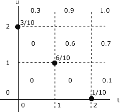
In Example 8.1.3 from "Random Vectors and Joint Distributions" we note that the joint distribution function \(F_{XY}\) is constant over any grid cell, including the left-hand and lower boundaries, at the value taken on at the lower left-hand corner of the cell. These lower left-hand corner values may be obtained systematically from the joint probability matrix P by a two step operation.
- Take cumulative sums upward of the columns of \(P\).
- Take cumulative sums of the rows of the resultant matrix.
This can be done with the MATLAB function cumsum, which takes column cumulative sums downward. By flipping the matrix and transposing, we can achieve the desired results.
Example 8.2.8: Calculation of FXY values for Example 8.3 from "Random Vectors and Joint Distributions"
>> P = 0.1*[3 0 0; 0 6 0; 0 0 1];
>> FXY = flipud(cumsum(flipud(P)))  % Cumulative column sums upward
FXY =
    0.3000    0.6000    0.1000
         0    0.6000    0.1000
         0         0    0.1000
>> FXY = cumsum(FXY')'              % Cumulative row sums
FXY =
    0.3000    0.9000    1.0000
         0    0.6000    0.7000
         0         0    0.1000

Comparison with Example 8.3 from "Random Vectors and Joint Distributions" shows agreement with values obtained by hand.
The two step procedure has been incorprated into an m-procedure jddbn. As an example, return to the distribution in Example Example 8.7
Example 8.2.9: Joint distribution function for example 8.7
>> jddbn
Enter joint probability matrix (as on the plane)  P
To view joint distribution function, call for FXY
>> disp(FXY)
    0.1512    0.3312    0.6012    0.7912    1.0000
    0.1152    0.2754    0.5157    0.6848    0.8756
    0.0780    0.1824    0.3390    0.4492    0.5656
    0.0264    0.0534    0.0939    0.1224    0.1356
These values may be put on a grid, in the same manner as in Figure 8.1.2 for Example 8.1.3 in "Random Vectors and Joint Distributions".
As in the case of canonic for a single random variable, it is often useful to have a function version of the procedure jcalc to provide the freedom to name the outputs conveniently. function[x,y,t,u,px,py,p] = jcalcf(X,Y,P) The quantities \(x, y, t, u, px, py\), and \(p\) may be given any desired names.
Joint absolutely continuous random variables
In the single-variable case, the condition that there are no point mass concentrations on the line ensures the existence of a probability density function, useful in probability calculations. A similar situation exists for a joint distribution for two (or more) variables. For any joint mapping to the plane which assigns zero probability to each set with zero area (discrete points, line or curve segments, and countable unions of these) there is a density function.
Definition
If the joint probability distribution for the pair \(\{X, Y\}\) assigns zero probability to every set of points with zero area, then there exists a joint density function \(f_{XY}\) with the property
\(P[(X, Y) \in Q] = \int \int_{Q} f_{XY}\)
We have three properties analogous to those for the single-variable case:
(f1) \(f_{XY} \ge 0\) (f2) \(\int \int_{R^2} f_{XY} = 1\) (f3) \(F_{XY} (t,u) = \int_{-\infty}^{1} \int_{-\infty}^{u} f_{XY}\)
At every continuity point for \(f_{XY}\), the density is the second partial
\(f_{XY} (t, u) = \dfrac{\partial^2 F_{XY} (t, u)}{\partial t \partial u}\)
Now
\(F_X (t) = F_{XY} (t, \infty) = \int_{-\infty}^{t} \int_{-\infty}^{\infty} f_{XY} (r, s) dsdr\)
A similar expression holds for \(F_Y(u)\). Use of the fundamental theorem of calculus to obtain the derivatives gives the result
\(f_X(t) = \int_{-\infty}^{\infty} f_{XY}(t, s) ds\) and \(f_Y(u) = \int_{-\infty}^{\infty} f_{XY} (r, u) du\)
Marginal densities. Thus, to obtain the marginal density for the first variable, integrate out the second variable in the joint density, and similarly for the marginal for the second variable.
Example 8.2.10: Marginal density functions
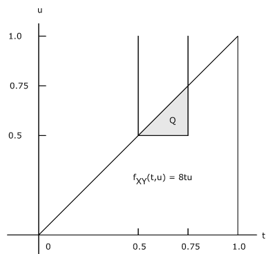
Let \(f_{XY} (t, u) = 8tu\) \(0 \le u \le t \le 1\). This region is the triangle bounded by \(u = 0, u = t\), and \(t = 1\)(see Figure 8.2.8)
\(f_X(t) = \int f_{XY} (t, u) du = 8t \int_{0}^{1} u du = 4t^3\), \(0 \le t \le 1\)
\(f_Y(u) = \int f_{XY} (t, u) dt = 8u \int_{u}^{1} t dt = 4u(1 - u^2)\), \(0 \le u \le 1\)
\(P(0.5 \le X \le 0.75, Y > 0.5) = P[(X, Y) \in Q]\) where \(Q\) is the common part of the triangle with the strip between \(t = 0.5\) and \(t = 0.75\) and above the line \(u = 0.5\). This is the small triangle bounded by \(u = 0.5\), \(u = t\), and \(t = 0.75\). Thus
\(p = 8 \int_{1/2}^{3/4} \int_{1/2}^{t} tu du dt = 25/256 \approx 0.0977\)

Example 8.2.11: Marginal distribution with compound expression
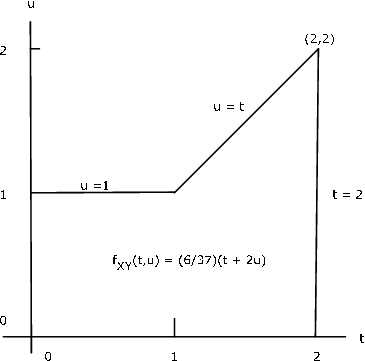
The pair \(\{X, Y\}\) has joint density \f_{XY}(t, u) = \dfrac{6}{37} (t + 2u)\) on the region bounded by \(t = 0, t = 2, u = 0\) and \(u = \text{max} \{1, t\}\) (see Figure 8.9). Determine the marginal density \(f_X\).
Solution
Examination of the figure shows that we have different limits for the integral with respect to \(u\) for \(0 \le t \le 1\) and for \(1 < t \le 2\).
- For \(0 \le t \le 1\)
\(f_x(t) = \dfrac{6}{37} \int_{0}^{1} (t + 2u) du = \dfrac{6}{37} (t + 1)\)
- For \(1 < t \le 2\)
\(f_X (t) = \dfrac{6}{37} \int_{0}^{1} (t + 2u) du = \dfrac{12}{37} t^2\)
We may combine these into a single expression in a manner used extensively in subsequent treatments. Suppose \(M = [0, 1]\) and \(N = (1, 2]\). Then \(I_M(t) = 1\) for \(t \in M\) (i.e., \(0 \le t \le 1\)) and zero elsewhere. Likewise, \(I_{N} (t) = 1\) for \(t \in N\) and zero elsewhere. We can, therefore express \(f_X\) by

Discrete approximation in the continuous case
For a pair \(\{X, Y\}\) with joint density \(f_{XY}\), we approximate the distribution in a manner similar to that for a single random variable. We then utilize the techniques developed for a pair of simple random variables. If we have \(n\) approximating values \(t_i\) for \(X\) and \(m\) approximating values \(u_j\) for \(Y\), we then have \(n \cdot m\) pairs \((t_i, u_j)\), corresponding to points on the plane. If we subdivide the horizontal axis for values of \(X\), with constant increments \(dx\), as in the single-variable case, and the vertical axis for values of \(Y\), with constant increments \(dy\), we have a grid structure consisting of rectangles of size \(dx \cdot dy\). We select \(t_i\) and \(u_j\) at the midpoint of its increment, so that the point \((t_i, u_j)\) is at the midpoint of the rectangle. If we let the approximating pair be \(\{X^*, Y^*\}\), we assign
\(p_{ij} = P((X^*, Y^*) = (t_i, u_j)) = P(X^* = t_i, Y^* = u_j) = P((X, Y) \text{ in } ij \text{th rectangle})\)
As in the one-variable case, if the increments are small enough,
\(P((X, Y) \in ij \text{th rectangle}) \approx dx \cdot dy \cdot f_{XY}(t_i, u_j)\)
The m-procedure tuappr calls for endpoints of intervals which include the ranges of \(X\) and \(Y\) and for the numbers of subintervals on each. It then prompts for an expression for \(f_{XY} (t, u)\), from which it determines the joint probability distribution. It calculates the marginal approximate distributions and sets up the calculating matrices \(t\) and \(u\) as does the m-process jcalc for simple random variables. Calculations are then carried out as for any joint simple pair.
Example 8.2.12: Approximation to a joint continuous distribution
\(f_{XY} (t, u) = 3\) on \(0 \le u \le t^2 \le 1\)
Determine \(P(X \le 0.8, Y > 0.1)\).
>> tuappr
Enter matrix [a b] of X-range endpoints  [0 1]
Enter matrix [c d] of Y-range endpoints  [0 1]
Enter number of X approximation points  200
Enter number of Y approximation points  200
Enter expression for joint density  3*(u <= t.^2)
Use array operations on X, Y, PX, PY, t, u, and P
>> M = (t <= 0.8)&(u > 0.1);
>> p = total(M.*P)          % Evaluation of the integral with
p =   0.3355                % Maple gives 0.3352455531
The discrete approximation may be used to obtain approximate plots of marginal distribution and density functions.

Example 8.2.13: Approximate plots of marginal density and distribution functions
\(f_{XY} (t, u) = 3u\) on the triangle bounded by \(u = 0\), \(u \le 1 + t\), and \(u \le 1 - t\).
>> tuappr
Enter matrix [a b] of X-range endpoints  [-1 1]
Enter matrix [c d] of Y-range endpoints  [0 1]
Enter number of X approximation points  400
Enter number of Y approximation points  200
Enter expression for joint density  3*u.*(u<=min(1+t,1-t))
Use array operations on X, Y, PX, PY, t, u, and P
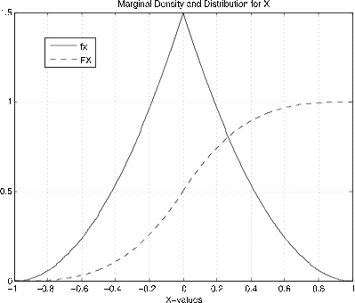
>> fx = PX/dx;                % Density for X  (see Figure 8.2.10)
                              % Theoretical (3/2)(1 - |t|)^2
>> fy = PY/dy;                % Density for Y
>> FX = cumsum(PX);           % Distribution function for X (Figure 8.2.10)
>> FY = cumsum(PY);           % Distribution function for Y
>> plot(X,fx,X,FX)            % Plotting details omitted
These approximation techniques useful in dealing with functions of random variables, expectations, and conditional expectation and regression.


