8.1: Random Vectors and Joint Distributions
- Page ID
- 10880

\( \newcommand{\vecs}[1]{\overset { \scriptstyle \rightharpoonup} {\mathbf{#1}} } \)
\( \newcommand{\vecd}[1]{\overset{-\!-\!\rightharpoonup}{\vphantom{a}\smash {#1}}} \)
\( \newcommand{\dsum}{\displaystyle\sum\limits} \)
\( \newcommand{\dint}{\displaystyle\int\limits} \)
\( \newcommand{\dlim}{\displaystyle\lim\limits} \)
\( \newcommand{\id}{\mathrm{id}}\) \( \newcommand{\Span}{\mathrm{span}}\)
( \newcommand{\kernel}{\mathrm{null}\,}\) \( \newcommand{\range}{\mathrm{range}\,}\)
\( \newcommand{\RealPart}{\mathrm{Re}}\) \( \newcommand{\ImaginaryPart}{\mathrm{Im}}\)
\( \newcommand{\Argument}{\mathrm{Arg}}\) \( \newcommand{\norm}[1]{\| #1 \|}\)
\( \newcommand{\inner}[2]{\langle #1, #2 \rangle}\)
\( \newcommand{\Span}{\mathrm{span}}\)
\( \newcommand{\id}{\mathrm{id}}\)
\( \newcommand{\Span}{\mathrm{span}}\)
\( \newcommand{\kernel}{\mathrm{null}\,}\)
\( \newcommand{\range}{\mathrm{range}\,}\)
\( \newcommand{\RealPart}{\mathrm{Re}}\)
\( \newcommand{\ImaginaryPart}{\mathrm{Im}}\)
\( \newcommand{\Argument}{\mathrm{Arg}}\)
\( \newcommand{\norm}[1]{\| #1 \|}\)
\( \newcommand{\inner}[2]{\langle #1, #2 \rangle}\)
\( \newcommand{\Span}{\mathrm{span}}\) \( \newcommand{\AA}{\unicode[.8,0]{x212B}}\)
\( \newcommand{\vectorA}[1]{\vec{#1}} % arrow\)
\( \newcommand{\vectorAt}[1]{\vec{\text{#1}}} % arrow\)
\( \newcommand{\vectorB}[1]{\overset { \scriptstyle \rightharpoonup} {\mathbf{#1}} } \)
\( \newcommand{\vectorC}[1]{\textbf{#1}} \)
\( \newcommand{\vectorD}[1]{\overrightarrow{#1}} \)
\( \newcommand{\vectorDt}[1]{\overrightarrow{\text{#1}}} \)
\( \newcommand{\vectE}[1]{\overset{-\!-\!\rightharpoonup}{\vphantom{a}\smash{\mathbf {#1}}}} \)
\( \newcommand{\vecs}[1]{\overset { \scriptstyle \rightharpoonup} {\mathbf{#1}} } \)
\(\newcommand{\longvect}{\overrightarrow}\)
\( \newcommand{\vecd}[1]{\overset{-\!-\!\rightharpoonup}{\vphantom{a}\smash {#1}}} \)
\(\newcommand{\avec}{\mathbf a}\) \(\newcommand{\bvec}{\mathbf b}\) \(\newcommand{\cvec}{\mathbf c}\) \(\newcommand{\dvec}{\mathbf d}\) \(\newcommand{\dtil}{\widetilde{\mathbf d}}\) \(\newcommand{\evec}{\mathbf e}\) \(\newcommand{\fvec}{\mathbf f}\) \(\newcommand{\nvec}{\mathbf n}\) \(\newcommand{\pvec}{\mathbf p}\) \(\newcommand{\qvec}{\mathbf q}\) \(\newcommand{\svec}{\mathbf s}\) \(\newcommand{\tvec}{\mathbf t}\) \(\newcommand{\uvec}{\mathbf u}\) \(\newcommand{\vvec}{\mathbf v}\) \(\newcommand{\wvec}{\mathbf w}\) \(\newcommand{\xvec}{\mathbf x}\) \(\newcommand{\yvec}{\mathbf y}\) \(\newcommand{\zvec}{\mathbf z}\) \(\newcommand{\rvec}{\mathbf r}\) \(\newcommand{\mvec}{\mathbf m}\) \(\newcommand{\zerovec}{\mathbf 0}\) \(\newcommand{\onevec}{\mathbf 1}\) \(\newcommand{\real}{\mathbb R}\) \(\newcommand{\twovec}[2]{\left[\begin{array}{r}#1 \\ #2 \end{array}\right]}\) \(\newcommand{\ctwovec}[2]{\left[\begin{array}{c}#1 \\ #2 \end{array}\right]}\) \(\newcommand{\threevec}[3]{\left[\begin{array}{r}#1 \\ #2 \\ #3 \end{array}\right]}\) \(\newcommand{\cthreevec}[3]{\left[\begin{array}{c}#1 \\ #2 \\ #3 \end{array}\right]}\) \(\newcommand{\fourvec}[4]{\left[\begin{array}{r}#1 \\ #2 \\ #3 \\ #4 \end{array}\right]}\) \(\newcommand{\cfourvec}[4]{\left[\begin{array}{c}#1 \\ #2 \\ #3 \\ #4 \end{array}\right]}\) \(\newcommand{\fivevec}[5]{\left[\begin{array}{r}#1 \\ #2 \\ #3 \\ #4 \\ #5 \\ \end{array}\right]}\) \(\newcommand{\cfivevec}[5]{\left[\begin{array}{c}#1 \\ #2 \\ #3 \\ #4 \\ #5 \\ \end{array}\right]}\) \(\newcommand{\mattwo}[4]{\left[\begin{array}{rr}#1 \amp #2 \\ #3 \amp #4 \\ \end{array}\right]}\) \(\newcommand{\laspan}[1]{\text{Span}\{#1\}}\) \(\newcommand{\bcal}{\cal B}\) \(\newcommand{\ccal}{\cal C}\) \(\newcommand{\scal}{\cal S}\) \(\newcommand{\wcal}{\cal W}\) \(\newcommand{\ecal}{\cal E}\) \(\newcommand{\coords}[2]{\left\{#1\right\}_{#2}}\) \(\newcommand{\gray}[1]{\color{gray}{#1}}\) \(\newcommand{\lgray}[1]{\color{lightgray}{#1}}\) \(\newcommand{\rank}{\operatorname{rank}}\) \(\newcommand{\row}{\text{Row}}\) \(\newcommand{\col}{\text{Col}}\) \(\renewcommand{\row}{\text{Row}}\) \(\newcommand{\nul}{\text{Nul}}\) \(\newcommand{\var}{\text{Var}}\) \(\newcommand{\corr}{\text{corr}}\) \(\newcommand{\len}[1]{\left|#1\right|}\) \(\newcommand{\bbar}{\overline{\bvec}}\) \(\newcommand{\bhat}{\widehat{\bvec}}\) \(\newcommand{\bperp}{\bvec^\perp}\) \(\newcommand{\xhat}{\widehat{\xvec}}\) \(\newcommand{\vhat}{\widehat{\vvec}}\) \(\newcommand{\uhat}{\widehat{\uvec}}\) \(\newcommand{\what}{\widehat{\wvec}}\) \(\newcommand{\Sighat}{\widehat{\Sigma}}\) \(\newcommand{\lt}{<}\) \(\newcommand{\gt}{>}\) \(\newcommand{\amp}{&}\) \(\definecolor{fillinmathshade}{gray}{0.9}\)A single, real-valued random variable is a function (mapping) from the basic space \(\Omega\) to the real line. That is, to each possible outcome \(\omega\) of an experiment there corresponds a real value \(t = X(\omega)\). The mapping induces a probability mass distribution on the real line, which provides a means of making probability calculations. The distribution is described by a distribution function \(F_X\). In the absolutely continuous case, with no point mass concentrations, the distribution may also be described by a probability density function \(f_X\). The probability density is the linear density of the probability mass along the real line (i.e., mass per unit length). The density is thus the derivative of the distribution function. For a simple random variable, the probability distribution consists of a point mass \(p_i\) at each possible value \(t_i\) of the random variable. Various m-procedures and m-functions aid calculations for simple distributions. In the absolutely continuous case, a simple approximation may be set up, so that calculations for the random variable are approximated by calculations on this simple distribution.
Often we have more than one random variable. Each can be considered separately, but usually they have some probabilistic ties which must be taken into account when they are considered jointly. We treat the joint case by considering the individual random variables as coordinates of a random vector. We extend the techniques for a single random variable to the multidimensional case. To simplify exposition and to keep calculations manageable, we consider a pair of random variables as coordinates of a two-dimensional random vector. The concepts and results extend directly to any finite number of random variables considered jointly.
Random variables considered jointly; random vectors
As a starting point, consider a simple example in which the probabilistic interaction between two random quantities is evident.
Example 8.1.1: A selection problem
Two campus jobs are open. Two juniors and three seniors apply. They seem equally qualified, so it is decided to select them by chance. Each combination of two is equally likely. Let \(X\) be the number of juniors selected (possible values 0, 1, 2) and \(Y\) be the number of seniors selected (possible values 0, 1, 2). However there are only three possible pairs of values for \((X, Y)\): (0, 2), (1, 1), or (2, 0). Others have zero probability, since they are impossible. Determine the probability for each of the possible pairs.
Solution
There are \(C(5, 2) = 10\) equally likely pairs. Only one pair can be both juniors. Six pairs can be one of each. There are \(C(3, 2) = 3\) ways to select pairs of seniors. Thus
\(P(X = 0, Y = 2) = 3/10\), \(P(X = 1, Y = 1) = 6/10\), \(P(X = 2, Y = 0) = 1/10\)
These probabilities add to one, as they must, since this exhausts the mutually exclusive possibilities. The probability of any other combination must be zero. We also have the distributions for the random variables conisidered individually.
\(X =\) [0 1 2] \(PX =\) [3/10 6/10 1/10] \(Y =\) [0 1 2] \(PY =\) [1/10 6/10 3/10]
We thus have a joint distribution and two individual or marginal distributions.
We formalize as follows:
A pair \(\{X, Y\}\) of random variables considered jointly is treated as the pair of coordinate functions for a two-dimensional random vector \(W = (X, Y)\). To each \(\omega \in \Omega\), \(W\) assigns the pair of real numbers \((t, u)\), where \(X(\omega) = t\) and \(Y(\omega) = u\). If we represent the pair of values \(\{t, u\}\) as the point \((t, u)\) on the plane, then \(W(\omega) = (t, u)\), so that
\(W = (X, Y): \Omega \to\) R\(^2\)
is a mapping from the basic space \(\Omega\) to the plane \(R^2\). Since \(W\) is a function, all mapping ideas extend. The inverse mapping \(W^{-1}\) plays a role analogous to that of the inverse mapping \(X^{-1}\) for a real random variable. A two-dimensional vector W is a random vector iff \(W^{-1}(Q)\) is an event for each reasonable set (technically, each Borel set) on the plane.
A fundamental result from measure theory ensures
\(W = (X, Y)\) is a random vector iff each of the coordinate functions \(X\) and \(Y\) is a random variable.
In the selection example above, we model \(X\) (the number of juniors selected) and \(Y\) (the number of seniors selected) as random variables. Hence the vector-valued function
Induced distribution and the joint distribution function
In a manner parallel to that for the single-variable case, we obtain a mapping of probability mass from the basic space to the plane. Since \(W^{-1}(Q)\) is an event for each reasonable set \(Q\) on the plane, we may assign to \(Q\) the probability mass
\(P_{XY} (Q) = P[W^{-1}(Q)] = P[(X, Y)^{-1} (Q)]\)
Because of the preservation of set operations by inverse mappings as in the single-variable case, the mass assignment determines \(P_{XY}\) as a probability measure on the subsets of the plane \(R^2\). The argument parallels that for the single-variable case. The result is the probability distribution induced by \(W = (X, Y)\). To determine the probability that the vector-valued function \(W = (X, Y)\) takes on a (vector) value in region \(Q\), we simply determine how much induced probability mass is in that region.
Example 8.1.2: Induced distribution and probability calculations
To determine \(P(1 \le X \le , Y > 0)\), we determine the region for which the first coordinate value (which we call \(t\)) is between one and three and the second coordinate value (which we call \(u\)) is greater than zero. This corresponds to the set \(Q\) of points on the plane with \(1 \le t \le 3\) and \(u > 0\). Geometrically, this is the strip on the plane bounded by (but not including) the horizontal axis and by the vertical lines \(t = 1\) and \(t = 3\)(included). The problem is to determine how much probability mass lies in that strip. How this is achieved depends upon the nature of the distribution and how it is described.
As in the single-variable case, we have a distribution function.
Definition: Joint Distribution Function
The joint distribution function \(F_{XY}\) for \(W = (X, Y)\) is given by
\[F_{XY} (t, u) = P(X \le t, Y \le u) \quad \forall (t, u) \in R^2\]
This means that \(F_{XY} (t, u)\) is equal to the probability mass in the region \(Q_{tu}\) on the plane such that the first coordinate is less than or equal to \(t\) and the second coordinate is less than or equal to \(u\). Formally, we may write
\(F_{XY} (t, u) = P[(X, Y) \in Q_{tu}]\), where \Q_{tu} = \{(r, s) : r \le t, s \le u\}\)
Now for a given point (\(a, b\)), the region \(Q_{ab}\) is the set of points (\(t, u\)) on the plane which are on or to the left of the vertical line through (\(t\), 0)and on or below the horizontal line through (0, \(u\)) (see Figure 1 for specific point \(t = a, u = b\)). We refer to such regions as semiinfinite intervals on the plane.
The theoretical result quoted in the real variable case extends to ensure that a distribution on the plane is determined uniquely by consistent assignments to the semiinfinite intervals \(Q_{tu}\). Thus, the induced distribution is determined completely by the joint distribution function.
Distribution function for a discrete random vector
The induced distribution consists of point masses. At point (\(t_i, u_j)\) in the range of \(W =(X, Y)\) there is probability mass \(P_{ij} = P[W = (t, u_j)] = P(X = t_i, Y = u_j)\). As in the general case, to determine \([P(X, Y) \in Q]\) we determine how much probability mass is in the region. In the discrete case (or in any case where there are point mass concentrations) one must be careful to note whether or not the boundaries are included in the region, should there be mass concentrations on the boundary.
Example 8.1.3: distribution function for the selection problem in Example 8.1.1
The probability distribution is quite simple. Mass 3/10 at (0,2), 6/10 at (1,1), and 1/10 at (2,0). This distribution is plotted in Figure 8.2. To determine (and visualize) the joint distribution function, think of moving the point \((t, u)\) on the plane. The region \Q_{tu}\) is a giant “sheet” with corner at \(t, u)\). The value of \(F_{XY} (t, u)\) is the amount of probability covered by the sheet. This value is constant over any grid cell, including the left-hand and lower boundariies, and is the value taken on at the lower left-hand corner of the cell. Thus, if \((t, u)\) is in any of the three squares on the lower left hand part of the diagram, no probability mass is covered by the sheet with corner in the cell. If \((t, u)\) is on or in the square having probability 6/10 at the lower left-hand corner, then the sheet covers that probability, and the value of \(F_{XY} (t, u) = 6/10\). The situation in the other cells may be checked out by this procedure.
Distribution function for a mixed distribution
Example 8.1.4: A Mixed Distribution
The pair \(\{X, Y\}\) produces a mixed distribution as follows (see Figure 8.3)
Point masses 1/10 at points (0,0), (1,0), (1,1), (0,1)
Mass 6/10 spread uniformly over the unit square with these vertices
The joint distribution function is zero in the second, third, and fourth quadrants.
- If the point \((t, u)\) is in the square or on the left and lower boundaries, the sheet covers the point mass at (0,0) plus 0.6 times the area covered within the square. Thus in this region
\(F_{XY} (t, u) = \dfrac{1}{10} (1 + 6tu)\)
- If the pont \((t, u)\) is above the square (including its upper boundary) but to the left of the line \(t = 1\), the sheet covers two point masses plus the portion of the mass in the square to the left of the vertical line through \((t, u)\). In this case
\(F_{XY} (t, u) = \dfrac{1}{10} (2 + 6t)\)
- If the point \((t, u)\) is to the right of the square (including its boundary) with \(0 \le u < 1\), the sheet covers two point masses and the portion of the mass in the square below the horizontal line through \((t, u)\), to give
F_{XY} (t, u) = \dfrac{1}{10} (2 + 6u)\)
- If \((t, u)\) is above and to the right of the square (i.e., both \(1 \le t\) and \(1 \le u\)). then all probability mass is covered and \(F_{XY} (t, u) = 1\) in this region.
Marginal Distributions
If the joint distribution for a random vector is known, then the distribution for each of the component random variables may be determined. These are known as marginal distributions. In general, the converse is not true. However, if the component random variables form an independent pair, the treatment in that case shows that the marginals determine the joint distribution.
To begin the investigation, note that
\(F_X (t) = P(X \le t) = P(X \le t, Y < \infty)\) i.e. \(Y\) can take any of its possible values.
Thus
\(F_X(t) = F_{XY}(t, \infty) = \text{lim}_{u \to \infty} F_{XY} (t, u)\)
This may be interpreted with the aid of Figure 8.1.4. Consider the sheet for point \((t, u)\).
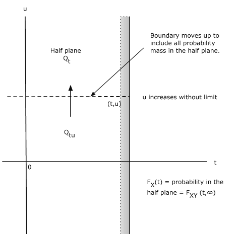
If we push the point up vertically, the upper boundary of \(Q_{tu}\) is pushed up until eventually all probability mass on or to the left of the vertical line through \((t, u)\) is included. This is the total probability that \(X \le t\). Now \(F_X(t)\) describes probability mass on the line. The probability mass described by \(F_X(t)\) is the same as the total joint probability mass on or to the left of the vertical line through \((t, u)\). We may think of the mass in the half plane being projected onto the horizontal line to give the marginal distribution for \(X\). A parallel argument holds for the marginal for \(Y\).
\(F_{Y} (u) = P(Y \le u) = F_{XY} (\infty, u) =\) mass on or below horizontal line through (\(t, u\))
This mass is projected onto the vertical axis to give the marginal distribution for \(Y\).
Marginals for a joint discrete distribution
Consider a joint simple distribution.
\(P(X = t_i) = \sum_{j = 1}^{m} P(X = t_i, Y = u_j) \) and \(P(Y = u_j) = \sum_{i = 1}^{n} P(X = t_i, Y = u_j)\)
Thus, all the probability mass on the vertical line through (\(t_i, 0\)) is projected onto the point \(t_i\) on a horizontal line to give \(P(X = t_i)\). Similarly, all the probability mass on a horizontal line through \((0, u_j)\) is projected onto the point \(u_j\) on a vertical line to give \(P(Y = u_j)\).
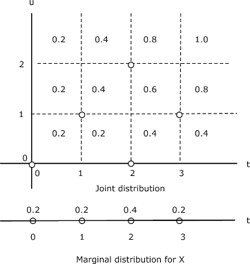
Example 8.1.5: Marginals for a discrete distribution
The pair \(\{X, Y\}\) produces a joint distribution that places mass 2/10 at each of the five points
(0, 0), (1, 1), (2, 0), (2, 2), (3, 1) (See Figure 8.1.5)
The marginal distribution for \(X\) has masses 2/10, 2/10, 4/10, 2/10 at points \(t = \) 0, 1, 2, 3, respectively. Similarly, the marginal distribution for Y has masses 4/10, 4/10, 2/10 at points \(u =\) 0, 1, 2, respectively.
Consider again the joint distribution in Example 8.4. The pair \(\{X, Y\}\) produces a mixed distribution as follows:
Point masses 1/10 at points (0,0), (1,0), (1,1), (0,1)
Mass 6/10 spread uniformly over the unit square with these vertices
The construction in Figure 8.1.6 shows the graph of the marginal distribution function \(F_X\). There is a jump in the amount of 0.2 at \(t = 0\), corresponding to the two point masses on the vertical line. Then the mass increases linearly with \(t\), slope 0.6, until a final jump at \(t = 1\) in the amount of 0.2 produced by the two point masses on the vertical line. At \(t = 1\), the total mass is “covered” and \(F_X(t)\) is constant at one for \(t \ge 1\). By symmetry, the marginal distribution for \(Y\) is the same.