7.2: Distribution Approximations

Binomial, Poisson, gamma, and Gaussian distributions

The Poisson approximation to the binomial distribution

The following approximation is a classical one. We wish to show that for small \(p\) and sufficiently large \(n\)

\[P(X = k) = C(n, k)p^k (1 - p)^{n - k} \approx e^{-np} \dfrac{np}{k!}\]

Suppose \(p = \mu/n\) with \(n\) large and \(\mu/n < 1\). Then,

\[P(X = k) = C(n, k) (\mu/n)^k (1 - \mu/n)^{n-k} = \dfrac{n(n - 1) \cdot \cdot \cdot (n - k + 1)}{n^k} (1 - \dfrac{\mu}{n})^{-k} (1 - \dfrac{\mu}{n})^n \dfrac{\mu^k}{k!}\]

The first factor in the last expression is the ratio of polynomials in \(n\) of the same degree \(k\), which must approach one as \(n\) becomes large. The second factor approaches one as \(n\) becomes large. According to a well known property of the exponential

\[(1 - \dfrac{\mu}{n})^n \to e^{-\mu}\]

as \(n \to \infty\).

The result is that for large \(n\), \(P(X = k) \approx e^{-\mu} \dfrac{\mu^k}{k!}\), where \(\mu = np\).

The Poisson and Gamma Distributions

Suppose \(Y~\) Poisson (\(\lambda t\)). Now \(X~\) gamma (\(\alpha, \lambda\)) iff

\[P(X \le t) = \dfrac{\lambda^{\alpha}}{\Gamma (\alpha)} \int_{0}^{1} x^{\alpha - 1} e^{-\lambda x}\ dx = \dfrac{1}{\Gamma (\alpha)} \int_{0}^{t} (\lambda x)^{\alpha - 1} e^{\lambda x} d(\lambda x) = \dfrac{1}{\Gamma (\alpha)} \int_{0}^{\lambda t} u^{\alpha - 1} e^{-\mu}\ du\]

A well known definite integral, obtained by integration by parts, is

\[int_{\alpha}^{\infty} t^{n -1} e^{-t}dt = \Gamma (n) e^{-a} \sum_{k = 1}^{n - 1} \dfrac{a^k}{k!}\]

with \(\Gamma (n) = (n - 1)!\).

Noting that \(1 = e^{-a}e^{a} = e^{-a} \sum_{k = 0}^{\infty} \dfrac{a^k}{k!}\) we find after some simple algebra that

\[\dfrac{1}{\Gamma(n)} \int_{0}^{a} t^{n -1} e^{-t}\ dt = e^{-a} \sum_{k = n}^{\infty} \dfrac{a^k}{k!}\]

For \(a = \lambda t\) and \(\alpha = n\), we have the following equality iff \(X~\) gamma (\(\alpha, \lambda\))

\[P(X \le t) = \dfrac{1}{\Gamma(n)} \int_{0}^{\lambda t} u^{n -1}d^{-u}\ du = e^{-\lambda t} \sum_{k = n}^{\infty} \dfrac{(\lambda t)^k}{k!}\]

Now

\[P(Y \ge n) = e^{-\lambda t} \sum_{k = n}^{\infty} \dfrac{(\lambda t)^k}{k!}\]

iff \(Y~\) Poisson (\(\lambda t\).

The Gaussian (normal) approximation

The central limit theorem, referred to in the discussion of the Gaussian or normal distribution above, suggests that the binomial and Poisson distributions should be approximated by the Gaussian. The number of successes in n trials has the binomial (n,p) distribution. This random variable may be expressed

\[X = \sum_{i = 1}^{n} I_{E_i}\]

Since the mean value of \(X\) is \(np\) and the variance is \(npq\), the distribution should be approximately \(N(np, npq)\).

Figure 7.2.8. Gaussian approximation to the binomial.

Use of the generating function shows that the sum of independent Poisson random variables is Poisson. Now if \(X~) Poisson (\(\mu\)), then \(X\) may be considered the sum of \(n\) independent random variables, each Poisson (\(\mu/n\)). Since the mean value and the variance are both \(\mu\), it is reasonable to suppose that suppose that \(X\) is approximately \(N(\mu, \mu)\).

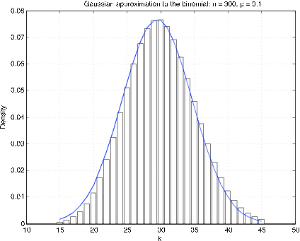
It is generally best to compare distribution functions. Since the binomial and Poisson distributions are integer-valued, it turns out that the best Gaussian approximation is obtained by making a “continuity correction.” To get an approximation to a density for an integer-valued random variable, the probability at \(t = k\) is represented by a rectangle of height \(p_k\) and unit width, with \(k\) as the midpoint. Figure 1 shows a plot of the “density” and the corresponding Gaussian density for \(n = 300\), \(p = 0.1\). It is apparent that the Gaussian density is offset by approximately 1/2. To approximate the probability \(X \le k\), take the area under the curve from \(k\) + 1/2; this is called the continuity correction.

Use of m-procedures to compare

We have two m-procedures to make the comparisons. First, we consider approximation of the

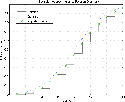
Figure 7.2.9. Gaussian approximation to the Poisson distribution function \(\mu\) = 10.

Figure 7.2.10. Gaussian approximation to the Poisson distribution function \(\mu\) = 100.

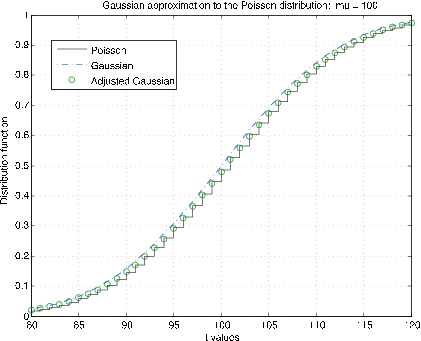
Poisson (\(\mu\)) distribution. The m-procedure poissapp calls for a value of \(\mu\), selects a suitable range about \(k = \mu\) and plots the distribution function for the Poisson distribution (stairs) and the normal (Gaussian) distribution (dash dot) for \(N(\mu, \mu)\). In addition, the continuity correction is applied to the gaussian distribution at integer values (circles). Figure 7.2.10 shows plots for \(\mu\) = 10. It is clear that the continuity correction provides a much better approximation. The plots in Figure 7.2.11 are for \(\mu\) = 100. Here the continuity correction provides the better approximation, but not by as much as for the smaller \(\mu\).

Figure 7.2.11. Poisson and Gaussian approximation to the binomial: \(n\) = 1000, \(p\) = 0.03.

Figure 7.2.12. Poisson and Gaussian approximation to the binomial: \(n\) = 50, \(p\) = 0.6.

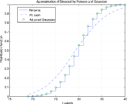
The m-procedure bincomp compares the binomial, gaussian, and Poisson distributions. It calls for values of \(n\) and \(p\), selects suitable \(k\) values, and plots the distribution function for the binomial, a continuous approximation to the distribution function for the Poisson, and continuity adjusted values of the gaussian distribution function at the integer values. Figure 7.2.11 shows plots for \(n = 1000\), \(p = 0.03\). The good agreement of all three distribution functions is evident. Figure 7.2.12 shows plots for \(n = 50, p = 0.6\). There is still good agreement of the binomial and adjusted gaussian. However, the Poisson distribution does not track very well. The difficulty, as we see in the unit Variance, is the difference in variances--\(npq\) for the binomial as compared with \(np\) for the Poisson.

Approximation of a real random variable by simple random variables

Simple random variables play a significant role, both in theory and applications. In the unit Random Variables, we show how a simple random variable is determined by the set of points on the real line representing the possible values and the corresponding set of probabilities that each of these values is taken on. This describes the distribution of the random variable and makes possible calculations of event probabilities and parameters for the distribution.

A continuous random variable is characterized by a set of possible values spread continuously over an interval or collection of intervals. In this case, the probability is also spread smoothly. The distribution is described by a probability density function, whose value at any point indicates "the probability per unit length" near the point. A simple approximation is obtained by subdividing an interval which includes the range (the set of possible values) into small enough subintervals that the density is approximately constant over each subinterval. A point in each subinterval is selected and is assigned the probability mass in its subinterval. The combination of the selected points and the corresponding probabilities describes the distribution of an approximating simple random variable. Calculations based on this distribution approximate corresponding calculations on the continuous distribution.

Before examining a general approximation procedure which has significant consequences for later treatments, we consider some illustrative examples.

Example \(\PageIndex{10}\): Simple approximation to Poisson

A random variable with the Poisson distribution is unbounded. However, for a given parameter value μ, the probability for \(k \ge n\), \(n\) sufficiently large, is negligible. Experiment indicates \(n = \mu + 6\sqrt{\mu}\) (i.e., six standard deviations beyond the mean) is a reasonable value for \(5 \le \mu \le 200\).

Solution

>> mu = [5 10 20 30 40 50 70 100 150 200];
>> K = zeros(1,length(mu));
>> p = zeros(1,length(mu));
>> for i = 1:length(mu)
     K(i) = floor(mu(i)+ 6*sqrt(mu(i)));
     p(i) = cpoisson(mu(i),K(i));
end
>> disp([mu;K;p*1e6]')
    5.0000   18.0000    5.4163  % Residual probabilities are 0.000001
   10.0000   28.0000    2.2535  % times the numbers in the last column.
   20.0000   46.0000    0.4540  % K is the value of k needed to achieve
   30.0000   62.0000    0.2140  % the residual shown.
   40.0000   77.0000    0.1354  
   50.0000   92.0000    0.0668
   70.0000  120.0000    0.0359
  100.0000  160.0000    0.0205
  150.0000  223.0000    0.0159
  200.0000  284.0000    0.0133

An m-procedure for discrete approximation

If \(X\) is bounded, absolutely continuous with density functon \(f_X\), the m-procedure tappr sets up the distribution for an approximating simple random variable. An interval containing the range of \(X\) is divided into a specified number of equal subdivisions. The probability mass for each subinterval is assigned to the midpoint. If \(dx\) is the length of the subintervals, then the integral of the density function over the subinterval is approximated by \(f_X(t_i) dx\). where \(t_i\) is the midpoint. In effect, the graph of the density over the subinterval is approximated by a rectangle of length \(dx\) and height \(f_X(t_i)\). Once the approximating simple distribution is established, calculations are carried out as for simple random variables.

Example \(\PageIndex{11}\): a numerical example

Suppose \(f_X(t) = 3t^2\), \(0 \le t \le 1\). Determine \(P(0.2 \le X \le 0.9)\).

Solution

In this case, an analytical solution is easy. \(F_X(t) = t^3\) on the interval [0, 1], so

\(P = 0.9^3 - 0.2^3 = 0.7210\). We use tappr as follows.

>> tappr
Enter matrix [a b] of x-range endpoints  [0 1]
Enter number of x approximation points  200
Enter density as a function of t  3*t.^2
Use row matrices X and PX as in the simple case
>> M = (X >= 0.2)&(X <= 0.9);
>> p = M*PX'
p  =  0.7210

Because of the regularity of the density and the number of approximation points, the result agrees quite well with the theoretical value.

The next example is a more complex one. In particular, the distribution is not bounded. However, it is easy to determine a bound beyond which the probability is negligible.

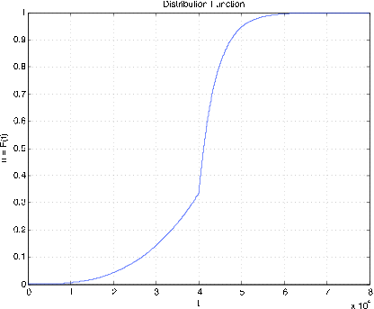
Figure 7.2.13. Distribution function for Example 7.2.12.

Example \(\PageIndex{12}\): Radial tire mileage

The life (in miles) of a certain brand of radial tires may be represented by a random variable \(X\) with density

\(f_X(t) = \begin{cases} t^2/a^3 & \text{for}\ \ 0 \le t < a \\ (b/a) e^{-k(t-a)} \text{for}\ \ a \le t \end{cases}\)

where \(a = 40,000\), \(b = 20/3\), and \(k = 1/4000\). Determine \(P(X \ge 45,000\).

>> a = 40000;
>> b = 20/3;
>> k = 1/4000;
>> % Test shows cutoff point of 80000 should be satisfactory
>> tappr
Enter matrix [a b] of x-range endpoints  [0 80000]
Enter number of x approximation points  80000/20
Enter density as a function of t  (t.^2/a^3).*(t < 40000) + ...
(b/a)*exp(k*(a-t)).*(t >= 40000)
Use row matrices X and PX as in the simple case
>> P = (X >= 45000)*PX'
P   =  0.1910             % Theoretical value = (2/3)exp(-5/4) = 0.191003
>> cdbn
Enter row matrix of VALUES  X
Enter row matrix of PROBABILITIES  PX  % See Figure 7.2.14 for plot

In this case, we use a rather large number of approximation points. As a consequence, the results are quite accurate. In the single-variable case, designating a large number of approximating points usually causes no computer memory problem.

The general approximation procedure

We show now that any bounded real random variable may be approximated as closely as desired by a simple random variable (i.e., one having a finite set of possible values). For the unbounded case, the approximation is close except in a portion of the range having arbitrarily small total probability.

We limit our discussion to the bounded case, in which the range of \(X\) is limited to a bounded interval \(I = [a, b]\). Suppose \(I\) is partitioned into \(n\) subintervals by points \(t_i\), \(1 \le i \le n - 1\), with \(a = t_0\) and \(b = t_n\). Let \(M_i = [t_{i- 1}, t_i)\) be the \(i\)th subinterval, \(1 \le i \le n - 1\) and \(M_n = [t_{n - 1}, t_n]\) (see Figure 7.14). Now random variable \(X\) may map into any point in the interval, and hence into any point in each subinterval \(M_i\). Let \(E_i X^{-1} (M_i)\) be the set of points mapped into \(M_i\) by \(X\). Then the \(E_i\) form a partition of the basic space \(\Omega\). For the given subdivision, we form a simple random variable \(X_s\) as follows. In each subinterval, pick a point \(s_i\), \(t_{i - 1} \le s_i \le t_i\). Consider the simple random variable \(X_s = \sum_{i = 1}^{n} s_i I_{E_i}\).

Figure 7.2.14. Partition of the interval \(I\) including the range of \(X\)

Figure 7.2.15. Refinement of the partition by additional subdividion points.

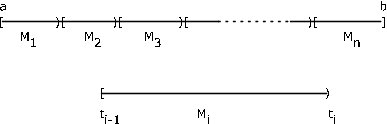
This random variable is in canonical form. If \(\omega \in E_i\), then \(X(\omega) \in M_i\) and \(X_s (\omega) = s_i\). Now the absolute value of the difference satisfies

\(|X(\omega) - X_s (\omega)| < t_i - t_{i - 1}\) the length of subinterval \(M_i\)

Since this is true for each \(\omega\) and the corresponding subinterval, we have the important fact

\(|X(\omega) - X_s (\omega)|<\) maximum length of the \(M_i\)

By making the subintervals small enough by increasing the number of subdivision points, we can make the difference as small as we please.

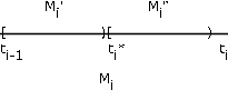
While the choice of the \(s_i\) is arbitrary in each \(M_i\), the selection of \(s_i = t_{i - 1}\) (the left-hand endpoint) leads to the property \(X_s(\omega) \le X(\omega) \forall \omega\). In this case, if we add subdivision points to decrease the size of some or all of the \(M_i\), the new simple approximation \(Y_s\) satisfies

\(X_s(\omega) = Y_s(\omega) \le X(\omega)\) \(\forall \omega\)

To see this, consider \(t_i^{*} \in M_i\)(see Figure 7.15). \(M_i\) is partitioned into \(M_i^{'} \bigcup M_i^{''}\) and \(E_i\) is partitioned into \(E_i^{'} \bigcup E_i^{''}\). \(X\) maps \(E_i^{'}\) into \(M_i^{'}\) and \(E_i^{''}\) into \(M_i^{''}\). \(Y_s\) maps \(E_i^{'}\) into \(t_i\) and maps \(E_i^{''}\) into \(t_i^{''}\) > t_i\). \(X_s\) maps both \(E_i^{'}\) and \(E_i^{''}\) into \(t_i\). Thus, the asserted inequality must hold for each \(\omega\) By taking a sequence of partitions in which each succeeding partition refines the previous (i.e. adds subdivision points) in such a way that the maximum length of subinterval goes to zero, we may form a nondecreasing sequence of simple random variables \(X_n\) which increase to \(X\) for each \(\omega\).

The latter result may be extended to random variables unbounded above. Simply let \(N\) th set of subdivision points extend from \(a\) to \(N\), making the last subinterval \([N, \infty)\). Subintervals from \(a\) to \(N\) are made increasingly shorter. The result is a nondecreasing sequence \(\{X_N: 1 \le N\}\) of simple random variables, with \(X_N(\omega) \to X(\omega)\) as \(N \to \infty\), for each \(\omega \in \Omega\).

For probability calculations, we simply select an interval \(I\) large enough that the probability outside \(I\) is negligible and use a simple approximation over \(I\).