7.1: Distribution and Density Functions

In the unit on Random Variables and Probability we introduce real random variables as mappings from the basic space \(\Omega\) to the real line. The mapping induces a transfer of the probability mass on the basic space to subsets of the real line in such a way that the probability that \(X\) takes a value in a set \(M\) is exactly the mass assigned to that set by the transfer. To perform probability calculations, we need to describe analytically the distribution on the line. For simple random variables this is easy. We have at each possible value of \(X\) a point mass equal to the probability \(X\) takes that value. For more general cases, we need a more useful description than that provided by the induced probability measure \(P_X\).

The Distribution Function

In the theoretical discussion on Random Variables and Probability, we note that the probability distribution induced by a random variable \(X\) is determined uniquely by a consistent assignment of mass to semi-infinite intervals of the form \((-\infty, t]\) for each real \(t\). This suggests that a natural description is provided by the following.

Definition

The distribution function \(F_X\) for random variable \(X\) is given by

\(F_X(t) P(X \le t) = P(X \in (-\infty, t])\) \(\forall t \in R\)

In terms of the mass distribution on the line, this is the probability mass at or to the left of the point t. As a consequence, \(F_X\) has the following properties:

• (F1) : \(F_X\) must be a nondecreasing function, for if \(t > s\) there must be at least as much probability mass at or to the left of \(t\) as there is for \(s\).
• (F2) : \(F_X\) is continuous from the right, with a jump in the amount \(p_0\) at \(t_0\) iff \(P(X = t_0) = p_0\). If the point \(t\) approaches \(t_0\) from the left, the interval does not include the probability mass at \(t_0\) until \(t\) reaches that value, at which point the amount at or to the left of t increases ("jumps") by amount \(p_0\); on the other hand, if \(t\) approaches \(t_0\) from the right, the interval includes the mass \(p_0\) all the way to and including \(t_0\), but drops immediately as \(t\) moves to the left of \(t_0\).
• (F3) : Except in very unusual cases involving random variables which may take “infinite” values, the probability mass included in \((-\infty, t]\) must increase to one as t moves to the right; as \(t\) moves to the left, the probability mass included must decrease to zero, so that \[F_X(-\infty) = \lim_{t \to - \infty} F_X(t) = 0\] and \[F_X(\infty) = \lim_{t \to \infty} F_X(t) = 1\]

A distribution function determines the probability mass in each semiinfinite interval \((\infty, t]\). According to the discussion referred to above, this determines uniquely the induced distribution.

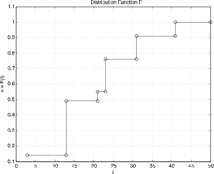
The distribution function \(F_X\) for a simple random variable is easily visualized. The distribution consists of point mass \(p_i\) at each point \(t_i\) in the range. To the left of the smallest value in the range, \(F_X(t) = 0\); as t increases to the smallest value \(t_1\), \(F_X(t)\) remains constant at zero until it jumps by the amount \(p_1\) ... \(F_X(t)\) remains constant at \(p_1\) until \(t\) increases to \(t_2\), where it jumps by an amount p₂ to the value \(p_1 + p_2\). This continues until the value of \(F_X(t)\) reaches 1 at the largest value \(t_n\). The graph of \(F_X\) is thus a step function, continuous from the right, with a jump in the amount \(p_i\) at the corresponding point \(t_i\) in the range. A similar situation exists for a discrete-valued random variable which may take on an infinity of values (e.g., the geometric distribution or the Poisson distribution considered below). In this case, there is always some probability at points to the right of any \(t_i\), but this must become vanishingly small as \(t\) increases, since the total probability mass is one.

The procedure ddbn may be used to plot the distribution function for a simple random variable from a matrix X of values and a corresponding matrix PX of probabilities.

Example \(\PageIndex{1}\): Graph of FX for a simple random variable

>> c = [10 18 10 3];             % Distribution for X in Example 6.5.1
>> pm = minprob(0.1*[6 3 5]);
>> canonic
 Enter row vector of coefficients  c
 Enter row vector of minterm probabilities  pm
Use row matrices X and PX for calculations
Call for XDBN to view the distribution
>> ddbn                          % Circles show values at jumps
Enter row matrix of VALUES  X
Enter row matrix of PROBABILITIES  PX
%  Printing details   See Figure 7.1

Figure 7.1.1. Distribution function for Example 7.1.1

Description of some common discrete distributions

We make repeated use of a number of common distributions which are used in many practical situations. This collection includes several distributions which are studied in the chapter "Random Variables and Probabilities".

Indicator function. \(X = I_E P(X = 1) = P(E) = pP(X = 0) = q = 1 - p\). The distribution function has a jump in the amount \(q\) at \(t = 0\) and an additional jump of \(p\) to the value 1 at \(t = 1\).

Simple random variable \(X = \sum_{t_i} I_{A_i}\) (canonical form)

\(P(X = t_i) = P(A_i) = p_1\)

The distribution function is a step function, continuous from the right, with jump of \(p_i\) at \(t = t_i\) (See Figure 7.1.1 for Example 7.1.1)

Binomial (\(n, p\)). This random variable appears as the number of successes in a sequence of \(n\) Bernoulli trials with probability \(p\) of success. In its simplest form

\(X = \sum_{i = 1}^{n} I_{E_i}\) with \(\{E_i: 1 \le i \le n\}\) independent

\(P(E_i) = p\) \(P(X = k) = C(n, k) p^k q^{n -k}\)

As pointed out in the study of Bernoulli sequences in the unit on Composite Trials, two m-functions ibinom andcbinom are available for computing the individual and cumulative binomial probabilities.

Geometric (\(p\)) There are two related distributions, both arising in the study of continuing Bernoulli sequences. The first counts the number of failures before the first success. This is sometimes called the “waiting time.” The event {\(X = k\)} consists of a sequence of \(k\) failures, then a success. Thus

\(P(X = k) = q^k p\), \(0 \le k\)

The second designates the component trial on which the first success occurs. The event {\(Y = k\)} consists of \(k - 1\) failures, then a success on the \(k\)th component trial. We have

\(P(Y = k) = q^{k - 1} p\), \(1 \le k\)

We say \(X\) has the geometric distribution with parameter (\(p\)), which we often designate by \(X~\) geometric (\(p\)). Now \(Y = X + 1\) or \(Y - 1 = X\). For this reason, it is customary to refer to the distribution for the number of the trial for the first success by saying \(Y - 1 ~\) geometric (\(p\)). The probability of \(k\) or more failures before the first success is \(P(X \ge k) = q^k\). Also

\(P(X \ge n + k| X \ge n) = \dfrac{P(X \ge n + k)}{P(X \ge n)} = q^{n + k}/q^{n} = q^k = P(X \ge k)\)

This suggests that a Bernoulli sequence essentially "starts over" on each trial. If it has failed \(n\) times, the probability of failing an additional \(k\) or more times before the next success is the same as the initial probability of failing \(k\) or more times before the first success.

Example \(\PageIndex{2}\): The geometric distribution

A statistician is taking a random sample from a population in which two percent of the members own a BMW automobile. She takes a sample of size 100. What is the probability of finding no BMW owners in the sample?

Solution

The sampling process may be viewed as a sequence of Bernoulli trials with probability \(p = 0.02\) of success. The probability of 100 or more failures before the first success is \(0.98^{100} = 0.1326\) or about 1/7.5.

Negative binomial (\(m, p\)). \(X\) is the number of failures before the \(m\)th success. It is generally more convenient to work with \(Y = X + m\), the number of the trial on which the \(m\)th success occurs. An examination of the possible patterns and elementary combinatorics show that

\(P(Y = k) = C(k - 1, m - 1) p^m q^{k - m}\), \(m \le k\)

There are m–1 successes in the first \(k - 1\) trials, then a success. Each combination has probability \(p^m q^{k - m}\). We have an m-function nbinom to calculate these probabilities.

Example \(\PageIndex{3}\): A game of chance

A player throws a single six-sided die repeatedly. He scores if he throws a 1 or a 6. What is the probability he scores five times in ten or fewer throws?

>> p = sum(nbinom(5,1/3,5:10))
p  =  0.2131

An alternate solution is possible with the use of the binomial distribution. The \(m\)th success comes not later than the kth trial iff the number of successes in \(k\) trials is greater than or equal to \(m\).

>> P = cbinom(10,1/3,5)
P  =  0.2131

Poisson (\(\mu\)). This distribution is assumed in a wide variety of applications. It appears as a counting variable for items arriving with exponential interarrival times (see the relationship to the gamma distribution below). For large \(n\) and small \(p\) (which may not be a value found in a table), the binomial distribution is approximately Poisson (\(np\)). Use of the generating function (see Transform Methods) shows the sum of independent Poisson random variables is Poisson. The Poisson distribution is integer valued, with

\(P(X = k) = e^{-\mu} \dfrac{\mu^k}{k!}\) (0 \le k\)

Although Poisson probabilities are usually easier to calculate with scientific calculators than binomial probabilities, the use of tables is often quite helpful. As in the case of the binomial distribution, we have two m-functions for calculating Poisson probabilities. These have advantages of speed and parameter range similar to those for ibinom and cbinom.

\(P(X = k)\) is calculated by P = ipoisson(mu,k), where \(k\) is a row or column vector of integers and the result \(P\) is a row matrix of the probabilities.
\(P(X \ge k)\) is calculated by P = cpoisson(mu,k), where \(k\) is a row or column vector of integers and the result \(P\) is a row matrix of the probabilities.

Example \(\PageIndex{4}\): Poisson counting random variable

The number of messages arriving in a one minute period at a communications network junction is a random variable N∼ Poisson (130). What is the probability the number of arrivals is greater than equal to 110, 120, 130, 140, 150, 160 ?

>> p = cpoisson(130,110:10:160)
p  =  0.9666  0.8209  0.5117  0.2011  0.0461  0.0060

The descriptions of these distributions, along with a number of other facts, are summarized in the table DATA ON SOME COMMON DISTRIBUTIONS in Appendix C.

The Density Function

If the probability mass in the induced distribution is spread smoothly along the real line, with no point mass concentrations, there is a probability density function \(f_X\) which satisfies

\(P(X \in M) = P_X(M) = \int_M f_X(t)\ dt\) (are under the graph of \(f_X\) over \(M\))

At each \(t\), \(f_X(t)\) is the mass per unit length in the probability distribution. The density function has three characteristic properties:

(f1) \(f_X \ge 0\) (f2) \(\int_R f_X = 1\) (f3) \(F_X (t) = \int_{-\infty}^{t} f_X\)

A random variable (or distribution) which has a density is called absolutely continuous. This term comes from measure theory. We often simply abbreviate as continuous distribution.

Remarks

1. There is a technical mathematical description of the condition “spread smoothly with no point mass concentrations.” And strictly speaking the integrals are Lebesgue integrals rather than the ordinary Riemann kind. But for practical cases, the two agree, so that we are free to use ordinary integration techniques.
2. By the fundamental theorem of calculus

   \(f_X(t) = F_X^{'} (t)\) at every point of continuity of \(f_X\)

• Any integrable, nonnegative function \(f\) with \(\int f = 1\) determines a distribution function \(F\), which in turn determines a probability distribution. If \(\int f \ne 1\), multiplication by the appropriate positive constant gives a suitable \(f\). An argument based on the Quantile Function shows the existence of a random variable with that distribution.
• In the literature on probability, it is customary to omit the indication of the region of integration when integrating over the whole line. Thus

  \(\int g(t) f_X (t) dt = \int_R g(t) f_X(t) dt\)

  The first expression is not an indefinite integral. In many situations, \(f_X\) will be zero outside an interval. Thus, the integrand effectively determines the region of integration.

Figure 7.1.2. The Weibull density for \(\alpha = 2\), \(\lambda = 0.25, 1, 4\).

Figure 7.1.3. The Weibull density for \(\alpha = 10\), \(\lambda = 0.001, 1, 1000\).

Some common absolutely continuous distributions

Uniform \((a, b)\).
Mass is spread uniformly on the interval \([a, b]\). It is immaterial whether or not the end points are included, since probability associated with each individual point is zero. The probability of any subinterval is proportional to the length of the subinterval. The probability of being in any two subintervals of the same length is the same. This distribution is used to model situations in which it is known that \(X\) takes on values in \([a, b]\) but is equally likely to be in any subinterval of a given length. The density must be constant over the interval (zero outside), and the distribution function increases linearly with \(t\) in the interval. Thus,

\(f_X (t) = \dfrac{1}{b - a}\) (\(a < t < b\)) (zero outside the interval)

The graph of \(F_X\) rises linearly, with slope 1/(\(b - a\)) from zero at \(t = a\) to one at \(t = b\).

Symmetric triangular \((-a, a)\), \(f_X(t) = \begin{cases} (a + t)/a^2 & -a \le t < 0 \\ (a - t)/a^2 & 0 \le t \le a \end{cases}\).
This distribution is used frequently in instructional numerical examples because probabilities can be obtained geometrically. It can be shifted, with a shift of the graph, to different sets of values. It appears naturally (in shifted form) as the distribution for the sum or difference of two independent random variables uniformly distributed on intervals of the same length. This fact is established with the use of the moment generating function (see Transform Methods). More generally, the density may have a triangular graph which is not symmetric.

Example \(\PageIndex{5}\): Use of a triangular distribution

Suppose \(X~\) symmetric triangular (100, 300). Determine \(P(120 < X \le 250)\).

Remark. Note that in the continuous case, it is immaterial whether the end point of the intervals are included or not.

Solution

To get the area under the triangle between 120 and 250, we take one minus the area of the right triangles between 100 and 120 and between 250 and 300. Using the fact that areas of similar triangles are proportional to the square of any side, we have

\(P = 1 - \dfrac{1}{2} ((20/100)^2 + (50/100)^2) = 0.855\)

Exponential (\(\lambda\)) \(f_X(t) = \lambda e^{-\lambda t}\) \(t \ge 0\) (zero elsewhere).
Integration shows \(F_X(t) = 1 - e^{-\lambda t}\) (t \ge 0\) (zero elsewhere). We note that \(P(X > 0) = 1 - F_X(t) = e^{-\lambda t}\) \(t \ge 0\). This leads to an extremely important property of the exponential distribution. Since \(X > t + h\), \(h > 0\) implies \(X > t\), we have

\(P(X > t + h|X > t) = P(X > t + h)/P(X > t) = e^{-\lambda (t+ h)}/e^{-\lambda t} = e^{-\lambda h} = P(X > h)\)

Because of this property, the exponential distribution is often used in reliability problems. Suppose \(X\) represents the time to failure (i.e., the life duration) of a device put into service at \(t = 0\). If the distribution is exponential, this property says that if the device survives to time \(t\) (i.e., \(X > t\)) then the (conditional) probability it will survive \(h\) more units of time is the same as the original probability of surviving for \(h\) units of time. Many devices have the property that they do not wear out. Failure is due to some stress of external origin. Many solid state electronic devices behave essentially in this way, once initial “burn in” tests have removed defective units. Use of Cauchy's equation (Appendix B) shows that the exponential distribution is the only continuous distribution with this property.

Gamma distribution \((\alpha, \lambda)\) \(f_X(t) = \dfrac{\lambda^{\alpha} t^{\alpha - 1} e^{-\lambda t}}{\Gamma (\alpha)}\) \(t \ge 0\) (zero elsewhere)
We have an m-function gammadbn to determine values of the distribution function for \(X~\) gamma \((\alpha, \lambda)\). Use of moment generating functions shows that for \(\alpha = n\), a random variable \(X~\) gamma \((n, \lambda)\) has the same distribution as the sum of \(n\) independent random variables, each exponential (\(lambda\)). A relation to the Poisson distribution is described in Sec 7.5.

Example \(\PageIndex{6}\): An arrival problem

On a Saturday night, the times (in hours) between arrivals in a hospital emergency unit may be represented by a random quantity which is exponential (\(\lambda = 3\)). As we show in the chapter Mathematical Expectation, this means that the average interarrival time is 1/3 hour or 20 minutes. What is the probability of ten or more arrivals in four hours? In six hours?

Solution

The time for ten arrivals is the sum of ten interarrival times. If we suppose these are independent, as is usually the case, then the time for ten arrivals is gamma (10, 3).

>> p = gammadbn(10,3,[4 6])
p  =  0.7576    0.9846

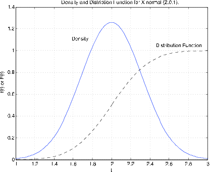
Normal, or Gaussian \((\mu, \sigma^2)\) \(f_X (t) = \dfrac{1}{\sigma \sqrt{2 \pi}}\) exp \((-\dfrac{1}{2} (\dfrac{t - \mu}{\sigma})^2)\) \(\forall t\)
We generally indicate that a random variable \(X\) has the normal or gaussian distribution by writing \(X ~ N(\mu, \sigma^2)\), putting in the actual values for the parameters. The gaussian distribution plays a central role in many aspects of applied probability theory, particularly in the area of statistics. Much of its importance comes from the central limit theorem (CLT), which is a term applied to a number of theorems in analysis. Essentially, the CLT shows that the distribution for the sum of a sufficiently large number of independent random variables has approximately the gaussian distribution. Thus, the gaussian distribution appears naturally in such topics as theory of errors or theory of noise, where the quantity observed is an additive combination of a large number of essentially independent quantities. Examination of the expression shows that the graph for \(f_X(t)\) is symmetric about its maximum at \(t = \mu\).. The greater the parameter \(\sigma^2\), the smaller the maximum value and the more slowly the curve decreases with distance from \(\mu\).. Thus parameter \(\mu\). locates the center of the mass distribution and \(\sigma^2\) is a measure of the spread of mass about \(\mu\). The parameter \(\mu\) is called the mean value and \(\sigma^2\) is the variance. The parameter \(\sigma\), the positive square root of the variance, is called the standard deviation. While we have an explicit formula for the density function, it is known that the distribution function, as the integral of the density function, cannot be expressed in terms of elementary functions. The usual procedure is to use tables obtained by numerical integration.
Since there are two parameters, this raises the question whether a separate table is needed for each pair of parameters. It is a remarkable fact that this is not the case. We need only have a table of the distribution function for \(X ~ N(0,1)\). This is refered to as the standardized normal distribution. We use \(\varphi\) and \(\phi\) for the standardized normal density and distribution functions, respectively.

Standardized normal \(varphi(t) = \dfrac{1}{\sqrt{2 \pi}} e^{-t^2/2}\) so that the distribution function is \(\phi (t) = \int_{-\infty}^{t} \varphi (u) du\).

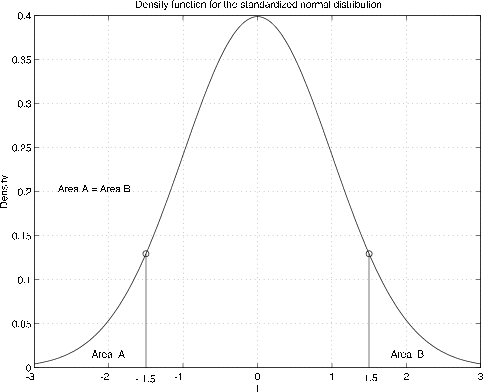
The graph of the density function is the well known bell shaped curve, symmetrical about the origin (see Figure 7.1.4). The symmetry about the origin contributes to its usefulness.

\(P(X \le t) = \phi (t)\) = area under the curve to the left of \(t\)

Note that the area to the left of \(t = -1.5\) is the same as the area to the right of \(t = 1.5\), so that \(\phi (-2) = 1 - \phi(2)\). The same is true for any \(t\), so that we have

\(\phi (-t) = 1 - \phi(t)\) \(\forall t\)

This indicates that we need only a table of values of \(\phi(t)\) for \(t > 0\) to be able to determine \(\phi (t)\) for any \(t\). We may use the symmetry for any case. Note that \(\phi(0) = 1/2\),

Figure 7.1.4. The standardized normal distribution.

Example \(\PageIndex{7}\): Standardized normal calculations

Suppose \(X ~ N(0, 1)\). Determine \(P(-1 \le X \le 2)\) and \(P(|X| > 1)\)

Solution

1. \(P(-1 \le X \le 2) = \phi (2) - \phi (-1) = \phi (2) - [1 - \phi(1)] = \phi (2) + \phi (1) - 1\)
2. \(P(|X| > 1) = P(X > 1) + P(X < -1) = 1 - \phi(1) + \phi (-1) = 2[1 -\phi(1)]\)

From a table of standardized normal distribution function (see Appendix D), we find

\(\phi(2) = 0.9772\) and \(\phi(1) = 0.8413\) which gives \(P(-1 \le X \le 2) = 0.8185\) and \(P(|X| > 1) = 0.3174\)

General gaussian distribution
For \(X~N(\mu, \sigma^2)\), the density maintains the bell shape, but is shifted with different spread and height. Figure 7.1.5 shows the distribution function and density function for \(X ~N(2, 0.1)\). The density is centered about \(t = 2\). It has height 1.2616 as compared with 0.3989 for the standardized normal density. Inspection shows that the graph is narrower than that for the standardized normal. The distribution function reaches 0.5 at the mean value 2.

Figure 7.1.5. The normal density and distribution functions for \(X ~N(2, 0.1)\).

A change of variables in the integral shows that the table for standardized normal distribution function can be used for any case.

\(F_X (t) = \dfrac{1}{\sigma \sqrt{2\pi}}\int_{-\infty}^{t} \text{exp}(-\dfrac{1}{2} (\dfrac{x - \mu}{\sigma})^2) dx = \int_{-infty}^{t} \varphi (\dfrac{x - \mu}{\sigma}) \dfrac{1}{\sigma} dx\)

Make the change of variable and corresponding formal changes

\(u = \dfrac{x - \mu}{\sigma}\) \(du = \dfrac{1}{\sigma} dx\) \(x = t ~ u = \dfrac{t - \mu}{\sigma}\)

to get

\(F_X(t) = \int_{-\infty}^{(t-\mu)/\sigma} \varphi (u) du = \phi (\dfrac{t - \mu}{\sigma})\)

Example \(\PageIndex{8}\): General gaussian calculation

Suppose \(X ~ N\)(3,16) (i.e., \(\mu = 3\) and \(\sigma^2 = 16\)). Determine \(P(-1 \le X \le 11)\) and \(P(|X - 3| > 4)\).

Solution

1. \(F_X(11) - F_X(-1) = \phi(\dfrac{11 - 3}{4}) - \phi(\dfrac{-1 - 3}{4}) = \phi(2) - \phi(-1) = 0.8185\)
2. \(P(X - 3 < -4) + P(X - 3 >4) = F_X(-1) + [1 - F_X(7)] = \phi(-1) + 1 - \phi(1) = 0.3174\)

In each case the problem reduces to that in Example.

We have m-functions gaussian and gaussdensity to calculate values of the distribution and density function for any reasonable value of the parameters.
The following are solutions of example 7.1.7 and example 7.1.8, using the m-function gaussian.

Example \(\PageIndex{9}\): Example 7.1.7 and Example 7.1.8 (continued)

>> P1 = gaussian(0,1,2) - gaussian(0,1,-1)
P1 =  0.8186
>> P2 = 2*(1 - gaussian(0,1,1))
P2 =  0.3173
>> P1 = gaussian(3,16,11) - gaussian(3,16,-1)
P2 =  0.8186
>> P2 = gaussian(3,16,-1)) + 1 - (gaussian(3,16,7)
P2 =  0.3173

The differences in these results and those above (which used tables) are due to the roundoff to four places in the tables.

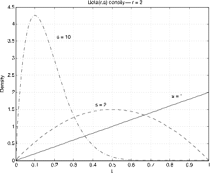
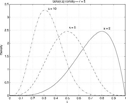
Beta \((r, s)\), \(r > 0\), \(s > 0\). \(f_X(t) = \dfrac{\Gamma(r + s)}{\Gamma(r) \Gamma(s)} t^{r - 1} (1 - t)^{s - 1}\) \(0 < t < 1\)

Analysis is based on the integrals

\(\int_{0}^{1} u^{r - 1} (1 - u)^{s - 1} du = \dfrac{\Gamma (r) \Gamma (s)}{\Gamma (r + s)}\) with \(\Gamma(t + 1) = t \Gamma (t)\)

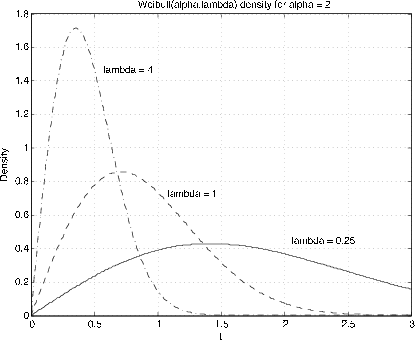
Figure 7.6 and Figure 7.7 show graphs of the densities for various values of \(r, s\). The usefulness comes in approximating densities on the unit interval. By using scaling and shifting, these can be extended to other intervals. The special case \(r = s = 1\) gives the uniform distribution on the unit interval. The Beta distribution is quite useful in developing the Bayesian statistics for the problem of sampling to determine a population proportion. If \(r, s\) are integers, the density function is a polynomial. For the general case we have two m-functions, beta and betadbn to perform the calculatons.

Figure 7.6. The Beta \((r, s)\) density for \(r = 2, s = 1, 2, 10\).

Figure 7.7. The Beta \((r, s)\) density for \(r = 5, s = 2, 5, 10\).

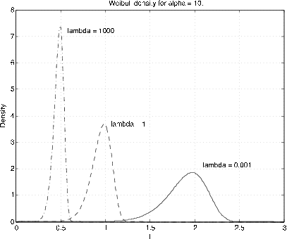
Weibull \((\alpha, \lambda, v)\) \(F_X (t) = 1 - e^{-\lambda (t - v)^{\alpha}}\) \(\alpha > 0\), \(\lambda > 0\), \(v \ge 0\), \(t \ge v\)
The parameter \(v\) is a shift parameter. Usually we assume \(v = 0\). Examination shows that for α=1 the distribution is exponential (\(\lambda\)). The parameter α provides a distortion of the time scale for the exponential distribution. Figure 7.6 and Figure 7.7 show graphs of the Weibull density for some representative values of \(\alpha\) and \(\lambda\) (\(v = 0\)). The distribution is used in reliability theory. We do not make much use of it. However, we have m-functions weibull (density) and weibulld (distribution function) for shift parameter \(v = 0\) only. The shift can be obtained by subtracting a constant from the \(t\) values.