28.6: Comparing More Than Two Means
- Page ID
- 8868
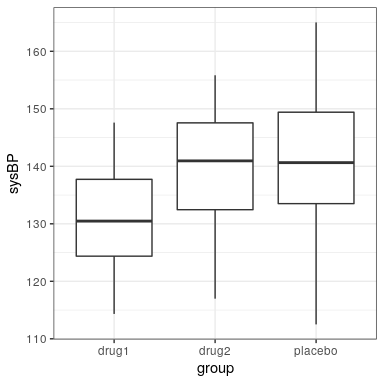
Often we want to compare more than two means to determine whether any of them differ from one another. Let’s say that we are analyzing data from a clinical trial for the treatment of high blood pressure. In the study, volunteers are randomized to one of three conditions: Drug 1, Drug 2 or placebo. Let’s generate some data and plot them (see Figure 28.4)

28.6.1 Analysis of variance
We would first like to test the null hypothesis that the means of all of the groups are equal – that is, neither of the treatments had any effect. We can do this using a method called analysis of variance (ANOVA). This is one of the most commonly used methods in psychological statistics, and we will only scratch the surface here. The basic idea behind ANOVA is one that we already discussed in the chapter on the general linear model, and in fact ANOVA is just a name for a specific implementation of such a model.
Remember from the last chapter that we can partition the total variance in the data () into the variance that is explained by the model () and the variance that is not (). We can then compute a mean square for each of these by dividing them by their degrees of freedom; for the error this is (where is the number of means that we have computed), and for the model this is :
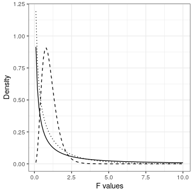
With ANOVA, we want to test whether the variance accounted for by the model is greater than what we would expect by chance, under the null hypothesis of no differences between means. Whereas for the t distribution the expected value is zero under the null hypothesis, that’s not the case here, since sums of squares are always positive numbers. Fortunately, there is another standard distribution that describes how ratios of sums of squares are distributed under the null hypothesis: The F distribution (see figure 28.5). This distribution has two degrees of freedom, which correspond to the degrees of freedom for the numerator (which in this case is the model), and the denominator (which in this case is the error).

To create an ANOVA model, we extend the idea of dummy coding that you encountered in the last chapter. Remember that for the t-test comparing two means, we created a single dummy variable that took the value of 1 for one of the conditions and zero for the others. Here we extend that idea by creating two dummy variables, one that codes for the Drug 1 condition and the other that codes for the Drug 2 condition. Just as in the t-test, we will have one condition (in this case, placebo) that doesn’t have a dummy variable, and thus represents the baseline against which the others are compared; its mean defines the intercept of the model. Let’s create the dummy coding for drugs 1 and 2.
Now we can fit a model using the same approach that we used in the previous chapter:
##
## Call:
## lm(formula = sysBP ~ d1 + d2, data = df)
##
## Residuals:
##     Min      1Q  Median      3Q     Max
## -29.084  -7.745  -0.098   7.687  23.431
##
## Coefficients:
##             Estimate Std. Error t value Pr(>|t|)
## (Intercept)   141.60       1.66   85.50  < 2e-16 ***
## d1            -10.24       2.34   -4.37  2.9e-05 ***
## d2             -2.03       2.34   -0.87     0.39
## ---
## Signif. codes:  0 '***' 0.001 '**' 0.01 '*' 0.05 '.' 0.1 ' ' 1
##
## Residual standard error: 9.9 on 105 degrees of freedom
## Multiple R-squared:  0.169,  Adjusted R-squared:  0.154
## F-statistic: 10.7 on 2 and 105 DF,  p-value: 5.83e-05
The output from this command provides us with two things. First, it shows us the result of a t-test for each of the dummy variables, which basically tell us whether each of the conditions separately differs from placebo; it appears that Drug 1 does whereas Drug 2 does not. However, keep in mind that if we wanted to interpret these tests, we would need to correct the p-values to account for the fact that we have done multiple hypothesis tests; we will see an example of how to do this in the next chapter.
Remember that the hypothesis that we started out wanting to test was whether there was any difference between any of the conditions; we refer to this as an omnibus hypothesis test, and it is the test that is provided by the F statistic. The F statistic basically tells us whether our model is better than a simple model that just includes an intercept. In this case we see that the F test is highly significant, consistent with our impression that there did seem to be differences between the groups (which in fact we know there were, because we created the data).


