28.5: Comparing Paired Observations

Figure 28.2: Left: Violin plot of systolic blood pressure on first and second recording, from NHANES. Right: Same violin plot with lines connecting the two data points for each individual.

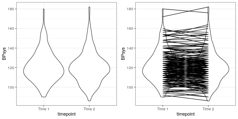
In experimental research, we often use within-subjects designs, in which we compare the same person on multiple measurements. The measurement that come from this kind of design are often referred to as repeated measures. For example, in the NHANES dataset blood pressure was measured three times. Let’s say that we are interested in testing whether there is a difference in mean blood pressure between the first and second measurement (Figure 28.2). We see that there does not seem to be much of a difference in mean blood pressure between time points (about one point). First let’s test for a difference using an independent samples t-test, which ignores the fact that pairs of data points come from the the same individuals.

## 
##  Two Sample t-test
## 
## data:  BPsys by timepoint
## t = 0.6, df = 398, p-value = 0.5
## alternative hypothesis: true difference in means is not equal to 0
## 95 percent confidence interval:
##  -2.1  4.1
## sample estimates:
## mean in group BPSys1 mean in group BPSys2 
##                  121                  120

This analysis shows no significant difference. However, this analysis is inappropriate since it assumes that the two samples are independent, when in fact they are not, since the data come from the same individuals. We can plot the data with a line for each individual to show this (see Figure ??).

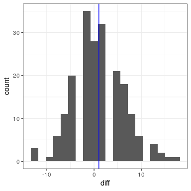
In this analysis, what we really care about is whether the blood pressure for each person changed in a systematic way between the two measurements, so another way to represent the data is to compute the difference between the two timepoints for each individual, and then analyze these difference scores rather than analyzing the individual measurements. In Figure 28.3, we show a histogram of these difference scores, with a blue line denoting the mean difference.

Figure 28.3: Histogram of difference scores between first and second BP measurement. The vertical line represents the mean difference in the sample.

28.5.1 Sign test

One simple way to test for differences is using the sign test. To do this, we take the differences and compute their sign, and then we use a binomial test to ask whether the proportion of positive signs differs from 0.5.

## 
##  Exact binomial test
## 
## data:  npos and nrow(NHANES_sample)
## number of successes = 96, number of trials = 200, p-value = 0.6
## alternative hypothesis: true probability of success is not equal to 0.5
## 95 percent confidence interval:
##  0.41 0.55
## sample estimates:
## probability of success 
##                   0.48

Here we see that the proportion of individuals with positive signs (0.48) is not large enough to be surprising under the null hypothesis of $p=0.5$. However, one problem with the sign test is that it is throwing away information about the magnitude of the differences, and thus might be missing something.

28.5.2 Paired t-test

A more common strategy is to use a paired t-test, which is equivalent to a one-sample t-test for whether the mean difference between the measurements is zero. We can compute this using the t.test() function in R and setting paired=TRUE.

## 
##  Paired t-test
## 
## data:  BPsys by timepoint
## t = 3, df = 199, p-value = 0.007
## alternative hypothesis: true difference in means is not equal to 0
## 95 percent confidence interval:
##  0.29 1.75
## sample estimates:
## mean of the differences 
##                       1

With this analyses we see that there is in fact a significant difference between the two measurements. Let’s compute the Bayes factor to see how much evidence is provided by the result:

## Bayes factor analysis
## --------------
## [1] Alt., r=0.707 : 3 ±0%
## 
## Against denominator:
##   Null, mu = 0 
## ---
## Bayes factor type: BFoneSample, JZS

This shows us that although the effect was significant in a paired t-test, it actually provides very little evidence in favor of the alternative hypothesis.

The paired t-test can also be defined in terms of a linear model; see the Appendix for more details on this.