27.3: Examples of Problematic Model Fit

Let’s say that there was another variable at play in this dataset, which we were not aware of. This variable causes some of the cases to have much larger values than others, in a way that is unrelated to the X variable. We play a trick here using the seq() function to create a sequence from zero to one, and then threshold those 0.5 (in order to obtain half of the values as zero and the other half as one) and then multiply by the desired effect size:

effsize=2
regression_data <- regression_data %>%
  mutate(y2=y + effsize*(seq(1/npoints,1,1/npoints)>0.5))

lm_result2 <- lm(y2 ~ x, data=regression_data)
summary(lm_result2)

## 
## Call:
## lm(formula = y2 ~ x, data = regression_data)
## 
## Residuals:
##     Min      1Q  Median      3Q     Max 
## -2.3324 -0.9689 -0.0939  1.0421  2.2591 
## 
## Coefficients:
##             Estimate Std. Error t value Pr(>|t|)    
## (Intercept)   10.978      0.117   93.65   <2e-16 ***
## x              0.270      0.119    2.27    0.025 *  
## ---
## Signif. codes:  0 '***' 0.001 '**' 0.01 '*' 0.05 '.' 0.1 ' ' 1
## 
## Residual standard error: 1.2 on 98 degrees of freedom
## Multiple R-squared:  0.0501, Adjusted R-squared:  0.0404 
## F-statistic: 5.17 on 1 and 98 DF,  p-value: 0.0252

One thing you should notice is that the model now fits overall much worse; the R-squared is about half of what it was in the previous model, which reflects the fact that more variability was added to the data, but it wasn’t accounted for in the model. Let’s see if our diagnostic reports can give us any insight:

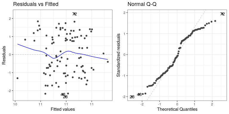
autoplot(lm_result2,which=1:2)

The residual versus fitted graph doesn’t give us much insight, but we see from the Q-Q plot that the residuals are diverging quite a bit from the unit line.

Let’s look at another potential problem, in which the y variable is nonlinearly related to the X variable. We can create these data by squaring the X variable when we generate the Y variable:

effsize=2
regression_data <- regression_data %>%
  mutate(y3 = (x**2)*slope + rnorm(npoints)*noise_sd + intercept)

lm_result3 <- lm(y3 ~ x, data=regression_data)
summary(lm_result3)

## 
## Call:
## lm(formula = y3 ~ x, data = regression_data)
## 
## Residuals:
##    Min     1Q Median     3Q    Max 
## -1.610 -0.568 -0.065  0.359  3.266 
## 
## Coefficients:
##             Estimate Std. Error t value Pr(>|t|)    
## (Intercept)  10.5547     0.0844  125.07   <2e-16 ***
## x            -0.0419     0.0854   -0.49     0.62    
## ---
## Signif. codes:  0 '***' 0.001 '**' 0.01 '*' 0.05 '.' 0.1 ' ' 1
## 
## Residual standard error: 0.84 on 98 degrees of freedom
## Multiple R-squared:  0.00245,    Adjusted R-squared:  -0.00773 
## F-statistic: 0.241 on 1 and 98 DF,  p-value: 0.625

Now we see that there is no significant linear relationship between $X$ and Y/ But if we look at the residuals the problem with the model becomes clear:

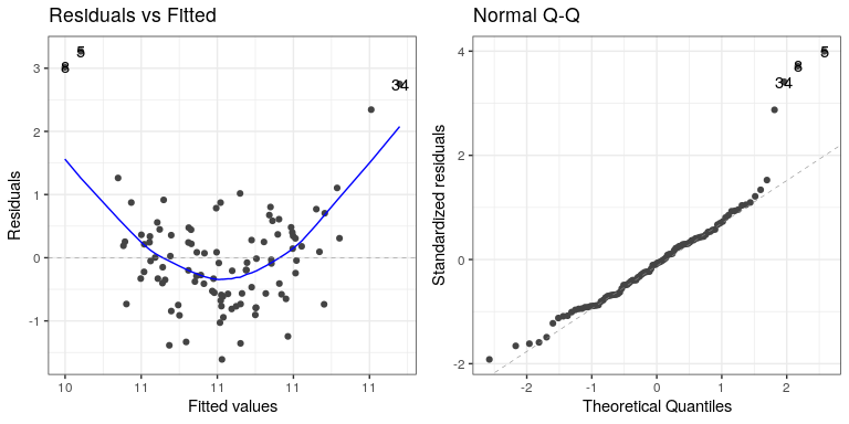
autoplot(lm_result3,which=1:2)

In this case we can see the clearly nonlinear relationship between the predicted and residual values, as well as the clear lack of normality in the residuals.

As we noted in the previous chapter, the “linear” in the general linear model doesn’t refer to the shape of the response, but instead refers to the fact that model is linear in its parameters — that is, the predictors in the model only get multiplied the parameters (e.g., rather than being raised to a power of the parameter). Here is how we would build a model that could account for the nonlinear relationship:

# create x^2 variable
regression_data <- regression_data %>%
  mutate(x_squared = x**2)

lm_result4 <- lm(y3 ~ x + x_squared, data=regression_data)
summary(lm_result4)

## 
## Call:
## lm(formula = y3 ~ x + x_squared, data = regression_data)
## 
## Residuals:
##     Min      1Q  Median      3Q     Max 
## -1.4101 -0.3791 -0.0048  0.3908  1.4437 
## 
## Coefficients:
##             Estimate Std. Error t value Pr(>|t|)    
## (Intercept)  10.1087     0.0739   136.8   <2e-16 ***
## x            -0.0118     0.0600    -0.2     0.84    
## x_squared     0.4557     0.0451    10.1   <2e-16 ***
## ---
## Signif. codes:  0 '***' 0.001 '**' 0.01 '*' 0.05 '.' 0.1 ' ' 1
## 
## Residual standard error: 0.59 on 97 degrees of freedom
## Multiple R-squared:  0.514,  Adjusted R-squared:  0.504 
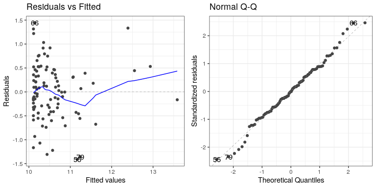
## F-statistic: 51.2 on 2 and 97 DF,  p-value: 6.54e-16

Now we see that the effect of $X$ is significant, and if we look at the residual plot we should see that things look much better:

autoplot(lm_result4,which=1:2)

Not perfect, but much better than before!