20.6: Bayesian Hypothesis Testing

Having learned how to perform Bayesian estimation, we now turn to the use of Bayesian methods for hypothesis testing. Let’s say that there are two politicians who differ in their beliefs about whether the public is in favor an extra tax to support the national parks. Senator Smith thinks that only 40% of people are in favor of the tax, whereas Senator Jones thinks that 60% of people are in favor. They arrange to have a poll done to test this, which asks 1000 randomly selected people whether they support such a tax. The results are that 490 of the people in the polled sample were in favor of the tax. Based on these data, we would like to know: Do the data support the claims of one senator over the other,and by how much? We can test this using a concept known as the Bayes factor,which quantifies which hypothesis is better by comparing how well each predicts the observed data.

20.6.1 Bayes factors

The Bayes factor characterizes the relative likelihood of the data under two different hypotheses. It is defined as:

$$BF = \frac{p(data|H_1)}{p(data|H_2)}$$

for two hypotheses $H$ and $H$. In the case of our two senators, we know how to compute the likelihood of the data under each hypothesis using the binomial distribution. We will put Senator Smith in the numerator and Senator Jones in the denominator, so that a value greater than one will reflect greater evidence for Senator Smith, and a value less than one will reflect greater evidence for Senator Jones. The resulting Bayes Factor (3325.26) provides a measure of the evidence that the data provides regarding the two hypotheses - in this case, it tells us the data support Senator Smith more than 3000 times more strongly than they support Senator Jones.

20.6.2 Bayes factors for statistical hypotheses

In the previous example we had specific predictions from each senator, whose likelihood we could quantify using the binomial distribution. However, in real data analysis we generally must deal with uncertainty about our parameters, which complicates the Bayes factor. However, in exchange we gain the ability to quantify the relative amount of evidence in favor of the null versus alternative hypotheses.

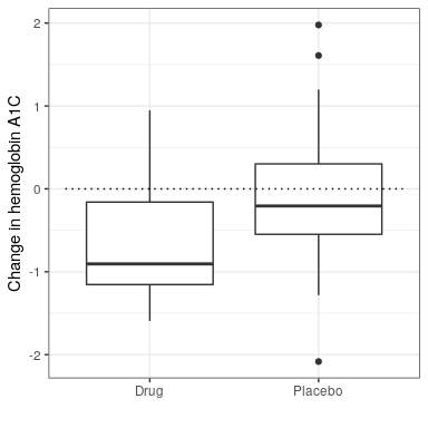
Let’s say that we are a medical researcher performing a clinical trial for the treatment of diabetes, and we wish to know whether a particular drug reduces blood glucose compared to placebo. We recruit a set of volunteers and randomly assign them to either drug or placebo group, and we measure the change in hemoglobin A1C (a marker for blood glucose levels) in each group over the period in which the drug or placebo was administered. What we want to know is: Is there a difference between the drug and placebo?

First, let’s generate some data and analyze them using null hypothesis testing (see Figure 20.5). Then let’s perform an independent-samples t-test, which shows that there is a significant difference between the groups:

Figure 20.5: Box plots showing data for drug and placebo groups.

## 
##  Welch Two Sample t-test
## 
## data:  hbchange by group
## t = 2, df = 32, p-value = 0.02
## alternative hypothesis: true difference in means is greater than 0
## 95 percent confidence interval:
##  0.11  Inf
## sample estimates:
## mean in group 0 mean in group 1 
##          -0.082          -0.650

This test tells us that there is a significant difference between the groups, but it doesn’t quantify how strongly the evidence supports the null versus alternative hypotheses. To measure that, we can compute a Bayes factor using ttestBF function from the BayesFactor package in R:

## Bayes factor analysis
## --------------
## [1] Alt., r=0.707 0<d<Inf    : 3.4  ±0%
## [2] Alt., r=0.707 !(0<d<Inf) : 0.12 ±0%
## 
## Against denominator:
##   Null, mu1-mu2 = 0 
## ---
## Bayes factor type: BFindepSample, JZS

We are particularly interested in the Bayes Factor for an effect greater than zero, which is listed in the line marked “[1]” in the report. The Bayes factor here tells us that the alternative hypothesis (i.e. that the difference is greater than zero) is about 3 times more likely than the point null hypothesis (i.e. a mean difference of exactly zero) given the data. Thus, while the effect is significant, the amount of evidence it provides us in favor of the alternative hypothesis is rather weak.

20.6.2.1 One-sided tests

We generally are less interested in testing against the null hypothesis of a specific point value (e.g. mean difference = 0) than we are in testing against a directional null hypothesis (e.g. that the difference is less than or equal to zero). We can also perform a directional (or one-sided) test using the results from ttestBF analysis, since it provides two Bayes factors: one for the alternative hypothesis that the mean difference is greater than zero, and one for the alternative hypothesis that the mean difference is less than zero. If we want to assess the relative evidence for a positive effect, we can compute a Bayes factor comparing the relative evidence for a positive versus a negative effect by simply dividing the two Bayes factors returned by the function:

## Bayes factor analysis
## --------------
## [1] Alt., r=0.707 0<d<Inf : 29 ±0%
## 
## Against denominator:
##   Alternative, r = 0.707106781186548, mu =/= 0 !(0<d<Inf) 
## ---
## Bayes factor type: BFindepSample, JZS

Now we see that the Bayes factor for a positive effect versus a negative effect is substantially larger (almost 30).

20.6.2.2 Interpreting Bayes Factors

How do we know whether a Bayes factor of 2 or 20 is good or bad? There is a general guideline for interpretation of Bayes factors suggested by Kass & Rafferty (1995):

BF	Strength of evidence
1 to 3	not worth more than a bare mention
3 to 20	positive
20 to 150	strong
>150	very strong

Based on this, even though the statisical result is significant, the amount of evidence in favor of the alternative vs. the point null hypothesis is weak enough that it’s not worth even mentioning, whereas the evidence for the directional hypothesis is relatively strong.

20.6.3 Assessing evidence for the null hypothesis

Because the Bayes factor is comparing evidence for two hypotheses, it also allows us to assess whether there is evidence in favor of the null hypothesis, which we couldn’t do with standard null hypothesis testing (because it starts with the assumption that the null is true). This can be very useful for determining whether a non-significant result really provides strong evidence that there is no effect, or instead just reflects weak evidence overall.