20.4: Estimating Posterior Distributions
- Page ID
- 8820
\( \newcommand{\vecs}[1]{\overset { \scriptstyle \rightharpoonup} {\mathbf{#1}} } \)
\( \newcommand{\vecd}[1]{\overset{-\!-\!\rightharpoonup}{\vphantom{a}\smash {#1}}} \)
\( \newcommand{\id}{\mathrm{id}}\) \( \newcommand{\Span}{\mathrm{span}}\)
( \newcommand{\kernel}{\mathrm{null}\,}\) \( \newcommand{\range}{\mathrm{range}\,}\)
\( \newcommand{\RealPart}{\mathrm{Re}}\) \( \newcommand{\ImaginaryPart}{\mathrm{Im}}\)
\( \newcommand{\Argument}{\mathrm{Arg}}\) \( \newcommand{\norm}[1]{\| #1 \|}\)
\( \newcommand{\inner}[2]{\langle #1, #2 \rangle}\)
\( \newcommand{\Span}{\mathrm{span}}\)
\( \newcommand{\id}{\mathrm{id}}\)
\( \newcommand{\Span}{\mathrm{span}}\)
\( \newcommand{\kernel}{\mathrm{null}\,}\)
\( \newcommand{\range}{\mathrm{range}\,}\)
\( \newcommand{\RealPart}{\mathrm{Re}}\)
\( \newcommand{\ImaginaryPart}{\mathrm{Im}}\)
\( \newcommand{\Argument}{\mathrm{Arg}}\)
\( \newcommand{\norm}[1]{\| #1 \|}\)
\( \newcommand{\inner}[2]{\langle #1, #2 \rangle}\)
\( \newcommand{\Span}{\mathrm{span}}\) \( \newcommand{\AA}{\unicode[.8,0]{x212B}}\)
\( \newcommand{\vectorA}[1]{\vec{#1}} % arrow\)
\( \newcommand{\vectorAt}[1]{\vec{\text{#1}}} % arrow\)
\( \newcommand{\vectorB}[1]{\overset { \scriptstyle \rightharpoonup} {\mathbf{#1}} } \)
\( \newcommand{\vectorC}[1]{\textbf{#1}} \)
\( \newcommand{\vectorD}[1]{\overrightarrow{#1}} \)
\( \newcommand{\vectorDt}[1]{\overrightarrow{\text{#1}}} \)
\( \newcommand{\vectE}[1]{\overset{-\!-\!\rightharpoonup}{\vphantom{a}\smash{\mathbf {#1}}}} \)
\( \newcommand{\vecs}[1]{\overset { \scriptstyle \rightharpoonup} {\mathbf{#1}} } \)
\( \newcommand{\vecd}[1]{\overset{-\!-\!\rightharpoonup}{\vphantom{a}\smash {#1}}} \)
\(\newcommand{\avec}{\mathbf a}\) \(\newcommand{\bvec}{\mathbf b}\) \(\newcommand{\cvec}{\mathbf c}\) \(\newcommand{\dvec}{\mathbf d}\) \(\newcommand{\dtil}{\widetilde{\mathbf d}}\) \(\newcommand{\evec}{\mathbf e}\) \(\newcommand{\fvec}{\mathbf f}\) \(\newcommand{\nvec}{\mathbf n}\) \(\newcommand{\pvec}{\mathbf p}\) \(\newcommand{\qvec}{\mathbf q}\) \(\newcommand{\svec}{\mathbf s}\) \(\newcommand{\tvec}{\mathbf t}\) \(\newcommand{\uvec}{\mathbf u}\) \(\newcommand{\vvec}{\mathbf v}\) \(\newcommand{\wvec}{\mathbf w}\) \(\newcommand{\xvec}{\mathbf x}\) \(\newcommand{\yvec}{\mathbf y}\) \(\newcommand{\zvec}{\mathbf z}\) \(\newcommand{\rvec}{\mathbf r}\) \(\newcommand{\mvec}{\mathbf m}\) \(\newcommand{\zerovec}{\mathbf 0}\) \(\newcommand{\onevec}{\mathbf 1}\) \(\newcommand{\real}{\mathbb R}\) \(\newcommand{\twovec}[2]{\left[\begin{array}{r}#1 \\ #2 \end{array}\right]}\) \(\newcommand{\ctwovec}[2]{\left[\begin{array}{c}#1 \\ #2 \end{array}\right]}\) \(\newcommand{\threevec}[3]{\left[\begin{array}{r}#1 \\ #2 \\ #3 \end{array}\right]}\) \(\newcommand{\cthreevec}[3]{\left[\begin{array}{c}#1 \\ #2 \\ #3 \end{array}\right]}\) \(\newcommand{\fourvec}[4]{\left[\begin{array}{r}#1 \\ #2 \\ #3 \\ #4 \end{array}\right]}\) \(\newcommand{\cfourvec}[4]{\left[\begin{array}{c}#1 \\ #2 \\ #3 \\ #4 \end{array}\right]}\) \(\newcommand{\fivevec}[5]{\left[\begin{array}{r}#1 \\ #2 \\ #3 \\ #4 \\ #5 \\ \end{array}\right]}\) \(\newcommand{\cfivevec}[5]{\left[\begin{array}{c}#1 \\ #2 \\ #3 \\ #4 \\ #5 \\ \end{array}\right]}\) \(\newcommand{\mattwo}[4]{\left[\begin{array}{rr}#1 \amp #2 \\ #3 \amp #4 \\ \end{array}\right]}\) \(\newcommand{\laspan}[1]{\text{Span}\{#1\}}\) \(\newcommand{\bcal}{\cal B}\) \(\newcommand{\ccal}{\cal C}\) \(\newcommand{\scal}{\cal S}\) \(\newcommand{\wcal}{\cal W}\) \(\newcommand{\ecal}{\cal E}\) \(\newcommand{\coords}[2]{\left\{#1\right\}_{#2}}\) \(\newcommand{\gray}[1]{\color{gray}{#1}}\) \(\newcommand{\lgray}[1]{\color{lightgray}{#1}}\) \(\newcommand{\rank}{\operatorname{rank}}\) \(\newcommand{\row}{\text{Row}}\) \(\newcommand{\col}{\text{Col}}\) \(\renewcommand{\row}{\text{Row}}\) \(\newcommand{\nul}{\text{Nul}}\) \(\newcommand{\var}{\text{Var}}\) \(\newcommand{\corr}{\text{corr}}\) \(\newcommand{\len}[1]{\left|#1\right|}\) \(\newcommand{\bbar}{\overline{\bvec}}\) \(\newcommand{\bhat}{\widehat{\bvec}}\) \(\newcommand{\bperp}{\bvec^\perp}\) \(\newcommand{\xhat}{\widehat{\xvec}}\) \(\newcommand{\vhat}{\widehat{\vvec}}\) \(\newcommand{\uhat}{\widehat{\uvec}}\) \(\newcommand{\what}{\widehat{\wvec}}\) \(\newcommand{\Sighat}{\widehat{\Sigma}}\) \(\newcommand{\lt}{<}\) \(\newcommand{\gt}{>}\) \(\newcommand{\amp}{&}\) \(\definecolor{fillinmathshade}{gray}{0.9}\)In the previous example there were only two possible outcomes – the explosive is either there or it’s not – and we wanted to know which outcome was most likely given the data. However, in other cases we want to use Bayesian estimation to estimate the numeric value of a parameter. Let’s say that we want to know about the effectiveness of a new drug for pain; to test this, we can administer the drug to a group of patients and then ask them whether their pain was improved or not after taking the drug. We can use Bayesian analysis to estimate the proportion of people for whom the drug will be effective using these data.
20.4.1 Specifying the prior
TBD: MH: USE PRIOR BIASED TOWARDS ZERO?
In this case, we don’t have any prior information about the effectiveness of the drug, so we will use a uniform distribution as our prior, since all values are equally likely under a uniform distribution. In order to simplify the example, we will only look at a subset of 99 possible values of effectiveness (from .01 to .99, in steps of .01). Therefore, each possible value has a prior probability of 1/99.
20.4.2 Collect some data
We need some data in order to estimate the effect of the drug. Let’s say that we administer the drug to 100 individuals, we find that 64 respond positively to the drug.
20.4.3 Computing the likelihood
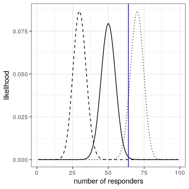
We can compute the likelihood of the data under any particular value of the effectiveness parameter using the dbinom() function in R. In Figure 20.2 you can see the likelihood curves over numbers of responders for several different values of . Looking at this, it seems that our observed data are relatively more likely under the hypothesis of , somewhat less likely under the hypothesis of , and quite unlikely under the hypothesis of . One of the fundamental ideas of Bayesian inference is that we should upweight our belief in values of our parameter of interest in proportion to how likely the data are under those values, balanced against what we believe about the parameter values before having seen the data (our prior knowledge).

20.4.4 Computing the marginal likelihood
In addition to the likelihood of the data under different hypotheses, we need to know the overall likelihood of the data, combining across all hypotheses (i.e., the marginal likelihood). This marginal likelihood is primarily important beacuse it helps to ensure that the posterior values are true probabilities. In this case, our use of a set of discrete possible parameter values makes it easy to compute the marginal likelihood, because we can just compute the likelihood of each parameter value under each hypothesis and add them up.
MH:not sure there’s a been clear discussion of the marginal likelihood up this point. it’s a confusing and also very deep construct.. the overall likelihood of the data is the likelihood of the data under each hypothesis, averaged togeteher (weifhted by) the prior probability of those hypotheses. it is how likely the data is under your prior beliefs about the hypotheses.
might be worth thinking of two examples, where the likelihood of the data under thet hypothesis of interest is the same, but where the marginal likelihood changes i.e., the hypothesis is pretty good at predicting the data, while other hypothese are bad vs. other hypotheses are always good (perhaps better)
20.4.5 Computing the posterior
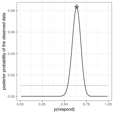
We now have all of the parts that we need to compute the posterior probability distribution across all possible values of

20.4.6 Maximum a posteriori (MAP) estimation
Given our data we would like to obtain an estimate of
20.4.7 Credible intervals
Often we would like to know not just a single estimate for the posterior, but an interval in which we are confident that the posterior falls. We previously discussed the concept of confidence intervals in the context of frequentist inference, and you may remember that the interpretation of confidence intervals was particularly convoluted: It was an interval that will contain the the value of the parameter 95% of the time. What we really want is an interval in which we are confident that the true parameter falls, and Bayesian statistics can give us such an interval, which we call a credible interval.
TBD: USE POSTERIOR FROM ABOVE
The interpretation of this credible interval is much closer to what we had hoped we could get from a confidence interval (but could not): It tells us that there is a 95% probability that the value of falls between these two values. Importantly, it shows that we have high confidence that , meaning that the drug seems to have a positive effect.
In some cases the credible interval can be computed numerically based on a known distribution, but it’s more common to generate a credible interval by sampling from the posterior distribution and then to compute quantiles of the samples. This is particularly useful when we don’t have an easy way to express the posterior distribution numerically, which is often the case in real Bayesian data analysis. One such method (rejection sampling) is explained in more detail in the Appendix at the end of this chapter.
20.4.8 Effects of different priors
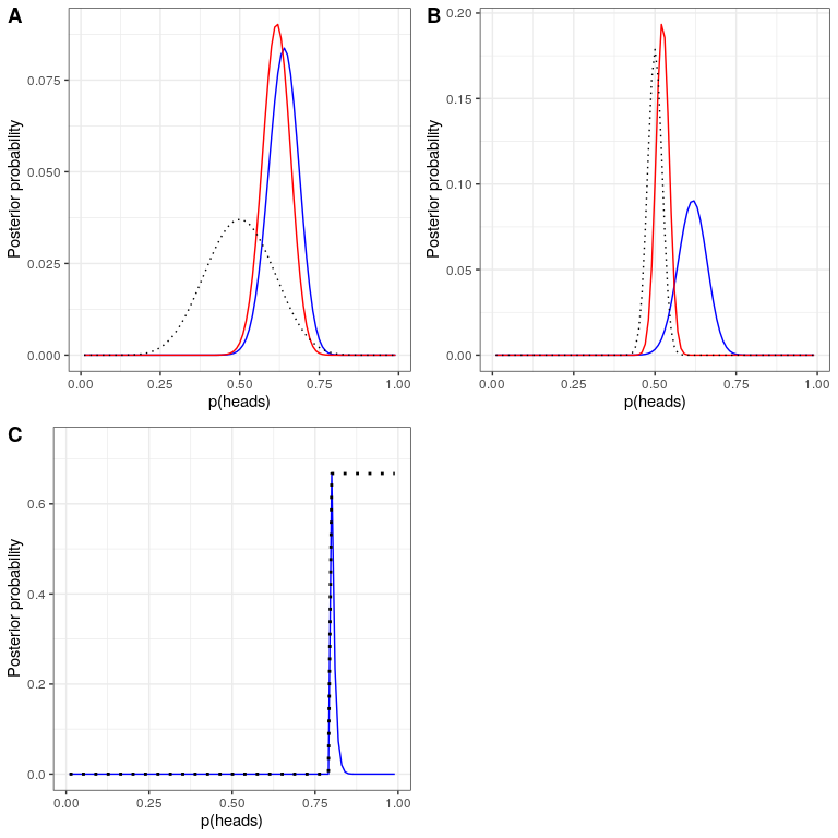
In the previous example we used a flat prior, meaning that we didn’t have any reason to believe that any particular value of was more or less likely. However, let’s say that we had instead started with some previous data: In a previous study, researchers had tested 20 people and found that 10 of them had responded positively. This would have lead us to start with a prior belief that the treatment has an effect in 50% of people. We can do the same computation as above, but using the information from our previous study to inform our prior (see oanel A in Figure 20.4).
MH: i wonder what you’re doing here: is this the same thing as doing a bayesian inference assuming 10 / 20 data and using the posterior from that as the prior for this analysis? that is what woud normally be the straightfoward thing to do.
Note that the likelihood and marginal likelihood did not change - only the prior changed. The effect of the change in prior to was to pull the posterior closer to the mass of the new prior, which is centered at 0.5.
Now let’s see what happens if we come to the analysis with an even stronger prior belief. Let’s say that instead of having previously observed 10 responders out of 20 people, the prior study had instead tested 500 people and found 250 responders. This should in principle give us a much stronger prior, and as we see in panel B of Figure 20.4 , that’s what happens: The prior is much more concentrated around 0.5, and the posterior is also much closer to the prior. The general idea is that Bayesian inference combines the information from the prior and the likelihood, weighting the relative strength of each.
This example also highlights the sequential nature of Bayesian analysis – the posterior from one analysis can become the prior for the next analysis.
Finally, it is important to realize that if the priors are strong enough, they can completely overwhelm the data. Let’s say that you have an absolute prior that is 0.8 or greater, such that you set the prior likelihood of all other values to zero. What happens if we then compute the posterior?

In panel C of Figure 20.4 we see that there is zero density in the posterior for any of the values where the prior was set to zero - the data are overwhelmed by the absolute prior.


