11.2: Pairwise Comparisons of Means (Post-Hoc Tests)

If you do in fact reject \(H_{0}\), then you know that at least two of the means are different. The ANOVA test does not tell which of those means are different, only that a difference exists. Most likely your sample means will be different from each other, but how different do they need to be for there to be a statistically significant difference?

To determine which means are significantly different, you need to conduct further tests. These post-hoc tests include the range test, multiple comparison tests, Duncan test, Student-Newman-Keuls test, Tukey test, Scheffé test, Dunnett test, Fisher’s least significant different test, and the Bonferroni test, to name a few. There are more options, and there is no consensus on which test to use. These tests are available in statistical software packages such as R, Minitab and SPSS.

One should never use two-sample \(t\)-tests from the previous chapter. This would inflate the type I error.

The probability of at least one type I error increases exponentially with the number of groups you are comparing. Let us assume that \(\alpha = 0.05\), then the probability that an observed difference between two groups that does not occur by chance is \(1 - \alpha = 0.95\). If two comparisons are made, the probability that the observed difference is true is no longer 0.95. The probability is \((1 - \alpha)^{2} = 0.9025\), and the P(Type I Error) = \(1 - 0.9025 = 0.0975\). Therefore, the P(Type I Error) occurs if \(m\) comparisons are made is \(1 - (1 - \alpha)m\).

For instance, if we are comparing the means of four groups: There would be \(m = {}_4 C_{2} = 6\) different ways to compare the 4 groups: groups (1,2), (1,3), (1,4), (2,3), (2,4), and (3,4). The P(Type I Error) = \(1 - (1 - \alpha)6 = 0.2649\). This is why a researcher should use ANOVA for comparing means, instead of independent \(t\)-tests.

There are many different methods to use. Many require special tables or software. We could actually just start with post-hoc tests, but they are a lot of work. If we run an ANOVA and we fail to reject the null hypothesis, then there is no need for further testing and it will save time if you were doing these steps by hand. Most statistical software packages give you the ANOVA table followed by the pairwise comparisons with just a change in the options menu. Keep in mind that Excel is not a statistical software and does not give pairwise comparisons.

We will use the Bonferroni Test, named after the mathematician Carlo Bonferroni. The Bonferroni Test uses the t-distribution table and is similar to previous t-tests that we have used, but adjusts \(\alpha\) to the number of comparisons being made.

Carlo Bonferroni

The Bonferroni test is a statistical test for testing the difference between two population means (only done after an ANOVA test shows not all means are equal).

The formula for the Bonferroni test statistic is \(t = \dfrac{\bar{x}_{i} - \bar{x}_{j}}{\sqrt{\left( MSW \left(\frac{1}{n_{i}} + \frac{1}{n_{j}}\right) \right)}}\).

where \(\bar{x}_{i}\) and \(\bar{x}_{j}\) are the means of the samples being compared, \(n_{i}\) and \(n_{j}\) are the sample sizes, and \(MSW\) is the within-group variance from the ANOVA table.

The Bonferroni test critical value or p-value is found by using the t-distribution with within degrees of freedom \(df_{W} = N-k\), using an adjusted \(\frac{\alpha}{m}\) two-tail area under the t-distribution, where \(k\) = number of groups and \(m = {}_{k} C_{2}\), all the combinations of pairs out of \(k\) groups.

Critical Value Method

According to the ANOVA test that we previously performed, there does appear to be a difference in the average age of assistant professors \((\mu_{1})\), associate professors \((\mu_{2})\), and full professors \((\mu_{3})\) at this university.

The hypotheses were:

\(H_{0}: \mu_{1} = \mu_{2} = \mu_{3}\)

\(H_{1}:\) At least one mean differs.

The decision was to reject \(H_{0}\), which means there is a significant difference in the mean age. The ANOVA test does not tell us, though, where the differences are. Determine which of the difference between each pair of means is significant. That is, test if \(\mu_{1} \neq \mu_{2}\), if \(\mu_{1} \neq \mu_{3}\), and if \(\mu_{2} \neq \mu_{3}\).

Solution

The alternative hypothesis for the ANOVA was “at least one mean is different.” There will be \({}_{3} C_{2} = 3\) subsequent hypothesis tests to compare all the combinations of pairs (Group 1 vs. Group 2, Group 1 vs. Group 3, and Group 2 vs. Group 3). Note that if you have 4 groups then you would have to do \({}_{4} C_{2} = 6\) comparisons, etc.

Use the t-distribution to find the critical value for the Bonferroni test. The total of all the individual sample sizes \(N = 21\) and \(k = 3\), and \(m = {}_{3} C_{2} = 3\), then the area for both tails would be \(\frac{\alpha}{m} = \frac{0.01}{m} = 0.003333\).

This is a two-tailed test so the area in one tail is \(\frac{0.003333}{2}\) with \(df_{W} = N-k = 21-3 = 18\) gives \(\text{C.V.} = \pm 3.3804\). The critical values are really far out in the tail so it is hard to see the shaded area. See Figure 11-3.

Figure 11-3: t-distribution with critical values.

Compare \(\mu_{1}\) and \(\mu_{2}\):

\(H_{0}: \mu_{1} = \mu_{2}\)

\(H_{1}: \mu_{1} \neq \mu_{2}\)

The test statistic is \(t = \frac{\bar{x}_{1} - \bar{x}_{2}}{\sqrt{\left( MSW \left(\frac{1}{n_{1}} + \frac{1}{n_{2}}\right) \right)}} = \frac{37 - 52}{\sqrt{\left(47.8889 \left(\frac{1}{7} + \frac{1}{7}\right) \right)}} = -4.0552\).

Compare the test statistic to the critical value. Since the test statistic \(-4.0552 < \text{critical value} = -3.3804\), we reject \(H_{0}\).

There is enough evidence to conclude that there is a difference in the average age of assistant and associate professors.

Compare \(\mu_{1}\) and \(\mu_{3}\):

\(H_{0}: \mu_{1} = \mu_{3}\)

\(H_{1}: \mu_{1} \neq \mu_{3}\)

The test statistic is \(t = \frac{\bar{x}_{1} - \bar{x}_{3}}{\sqrt{\left( MSW \left(\frac{1}{n_{1}} + \frac{1}{n_{3}}\right) \right)}} = \frac{37 - 54}{\sqrt{\left(47.8889 \left(\frac{1}{7} + \frac{1}{7}\right) \right)}} = -4.5958\).

Compare the test statistic to the critical value. Since the test statistic \(-4.5958 < \text{critical value} = -3.3804\), we reject \(H_{0}\).

Reject \(H_{0}\), since the test statistic is in the lower tail. There is enough evidence to conclude that there is a difference in the average age of assistant and full professors.

Compare \(\mu_{2}\) and \(\mu_{3}\):

\(H_{0}: \mu_{2} = \mu_{3}\)

\(H_{1}: \mu_{2} \neq \mu_{3}\)

The test statistic is \(t = \frac{\bar{x}_{2} - \bar{x}_{3}}{\sqrt{\left( MSW \left(\frac{1}{n_{2}} + \frac{1}{n_{3}}\right) \right)}} = \frac{52 - 54}{\sqrt{\left(47.8889 \left(\frac{1}{7} + \frac{1}{7}\right) \right)}} = -0.5407\)

Compare the test statistic to the critical value. Since the test statistic is between the critical values \(-3.3804 < -0.5407 < 3.3804\), we fail to reject \(H_{0}\).

Do not reject \(H_{0}\), since the test statistic is between the two critical values. There is enough evidence to conclude that there is not a difference in the average age of associate and full professors.

Note: you should get at least one group that has a reject \(H_{0}\), since you only do the Bonferroni test if you reject \(H_{0}\) for the ANOVA. Also, note that the transitive property does not apply. It could be that group 1 = group 2 and group 2 = group 3; this does not mean that group 1 = group 3.

P-Value Method

A research organization tested microwave ovens. At \(\alpha\) = 0.10, is there a significant difference in the average prices of the three types of oven?

Solution

The ANOVA was run in Excel.

To test if there is a significant difference in the average prices of the three types of oven, the hypotheses are:

\(H_{0}: \mu_{1} = \mu_{2} = \mu_{3}\)

\(H_{1}:\) At least one mean differs.

Use the Excel output to find the p-value in the ANOVA table of 0.001019, which is less than \(\alpha\) so reject \(H_{0}\); there is at least one mean that is different in the average oven prices.

There is a statistically significant difference in the average prices of the three types of oven. Use the Bonferroni test p-value method to see where the differences are.

Compare \(\mu_{1}\) and \(\mu_{2}\):

\(H_{0}: \mu_{1} = \mu_{2}\)

\(H_{1}: \mu_{1} \neq \mu_{2}\)

\(t = \frac{\bar{x}_{1} - \bar{x}_{2}}{\sqrt{\left( MSW \left(\frac{1}{n_{1}} + \frac{1}{n_{2}}\right) \right)}} = \frac{233.3333-203.125}{\sqrt{\left((1073.794 \left(\frac{1}{6} + \frac{1}{8}\right) \right)}} = 1.7070\)

To find the p-value, find the area in both tails and multiply this area by \(m\). The area to the right of \(t = 1.707\), using \(df_{W} = 19\), is 0.0520563. Remember these are always two-tail tests, so multiply this area by 2, to get both tail areas of 0.104113.

Then multiply this area by \(m = {}_{3} C_{2} = 3\) to get a p-value = 0.3123.

Since the p-value = \(0.3123 > \alpha = 0.10\), we do not reject \(H_{0}\). There is a statistically significant difference in the average price of the 1,000- and 900-watt ovens.

Compare \(\mu_{1}\) and \(\mu_{3}\):

\(H_{0}: \mu_{1} = \mu_{3}\)

\(H_{1}: \mu_{1} \neq \mu_{3}\)

\(t = \frac{\bar{x}_{1} - \bar{x}_{3}}{\sqrt{\left( MSW \left(\frac{1}{n_{1}} + \frac{1}{n_{3}}\right) \right)}} = \frac{233.3333-155.625}{\sqrt{\left((1073.794 \left(\frac{1}{6} + \frac{1}{8}\right) \right)}} = 4.3910\)

Use \(df_{W}\) = 19 to find the p-value.

Since the p-value = (tail areas)*3 = \(0.00094 < \alpha = 0.10\), we reject \(H_{0}\). There is a statistically significant difference in the average price of the 1,000- and 800-watt ovens.

Compare \(\mu_{2}\) and \(\mu_{3}\):

\(H_{0}: \mu_{2} = \mu_{3}\)

\(H_{1}: \mu_{2} \neq \mu_{3}\)

\(t = \frac{\bar{x}_{2} - \bar{x}_{3}}{\sqrt{\left( MSW \left(\frac{1}{n_{2}} + \frac{1}{n_{3}}\right) \right)}} = \frac{203.125-155.625}{\sqrt{\left((1073.794 \left(\frac{1}{8} + \frac{1}{8}\right) \right)}} = 2.8991\)

Use \(df_{W} = 19\) to find the p-value (remember that these are always two-tail tests).

Since the p-value = \(0.0276 < \alpha = 0.10\), we reject \(H_{0}\). There is a statistically significant difference in the average price of the 900- and 800-watt ovens.

There is a chance that after we multiply the area by the number of comparisons, the p-value would be greater than one. However, since the p-value is a probability we would cap the probability at one.

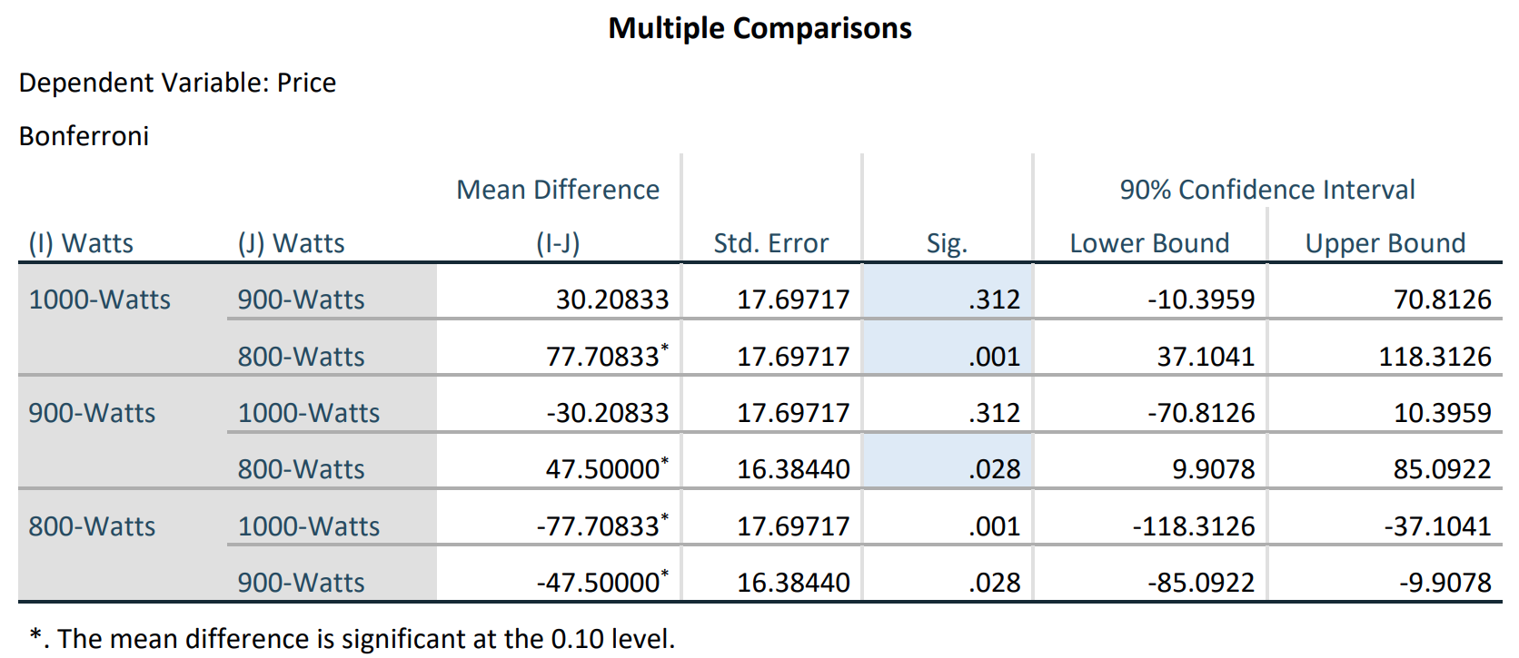
This is a lot of math! The calculators and Excel do not have post-hoc pairwise comparisons shortcuts, but we can use the statistical software called SPSS to get the following results. We will look specifically at interpreting the SPSS output for Example 11-4.

Figure 11-4: Multiple Comparisons table.

The first table, labeled "Descriptives", gives descriptive statistics; the second table is the ANOVA table, and note that the p-value is in the column labeled Sig. The Multiple Comparisons table is where we want to look. There are repetitive pairs in the last table, just in a different order.

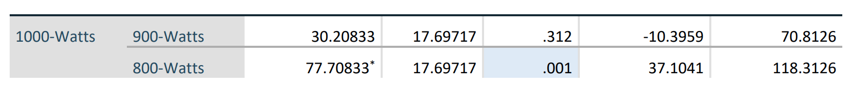
The first two rows in Figure 11-4 are comparing group 1 with groups 2 and 3. If we follow the first row across under the Sig. column, this gives the p-value = 0.312 for comparing the 1,000- and 900-watt ovens.

The second row in Figure 11-4 compares the 1,000- and 800-watt ovens, p-value = 0.001.

The third row in Figure 11-4 compares the 900- and 1000-watt ovens in the reverse order as the first row; note that the difference in the means is negative but the p-value is the same.

The fourth row in Figure 11-4 compares the 900- and 800-watt ovens, p-value = 0.028.

The last set of rows in Figure 11-4 are again repetitive and give the 800-watt oven compared to the 900- and 1000-watt ovens.

Keep in mind that post-hoc is defined as occurring after an event. A post-hoc test is done after an ANOVA test shows that there is a statistically significant difference. You should get at least one group that has a result of "reject \(H_{0}\)", since you only do the Bonferroni test if you reject \(H_{0}\) for the ANOVA.