
11.1: One-Way ANOVA
- Page ID
- 24071

The \(z\)- and \(t\)-tests can be used to test the equality between two population means \(\mu_{1}\) and \(\mu_{2}\). When we have more than two groups, we would inflate the probability of making a type I error if we were to compare just two at a time and make a conclusion about all the groups together. To account for this P(Type I Error) inflation, we instead will do an analysis of variance (ANOVA) to test the equality between 3 or more population means \(\mu_{1}, \mu_{2}, \mu_{3}, \ldots, \mu_{k}\).
The F-test (for ANOVA) is a statistical test for testing the equality of \(k\) population means.
The one-way ANOVA F-test is a statistical test for testing the equality of \(k\) population means from 3 or more groups within one variable or factor. There are many different types of ANOVA; for now, we are going to start with what is commonly referred to as a one-way ANOVA, which has one main effect or factor that is split up into three or more independent treatment levels. In more advanced courses you would learn about dependent groups or two or more factors.
Assumptions:
- The populations are normally distributed continuous variables with equal variances.
- The observations are independent.
The hypotheses for testing the equality of \(k\) population means (ANOVA) are set up with all the means equal to one another in the null hypothesis and at least one mean is different in the alternative hypothesis.
\(H_{0}: \mu_{1} = \mu_{2} = \mu_{3} = \ldots = \mu_{k}\)
\(H_{1}:\) At least one mean is different.
Even though there is equality in \(H_{0}\), the ANOVA test is testing if the variance between groups is significantly greater than the variance within groups; hence, this will always be set up as a right-tailed test.
We will be using abbreviations for many of the numbers found in this section.
B = Between, W = Within
MS = Mean Square (This is a variance)
MSB = Mean Square (Variance) Between groups.
MSW = Mean Square (Variance) Within groups.
The formula for the F-test statistic is \(F = \frac{MSB}{MSW}\).
Use the F-distribution with degrees of freedom from the between and within groups. The numerator degrees of freedom are equal to the number of groups minus one, that is numerator degrees of freedom are \(df_{B} = k - 1\). The denominator degrees of freedom are equal to the total of all the sample sizes minus the number of groups, that is denominator degrees of freedom are \(df_{W} = N - k\).
The sum of squares, degrees of freedom and mean squares are organized in a table called an ANOVA table. Figure 11-1 below is a template for an ANOVA table.
.png?revision=1)
Where:
\(\bar{\chi}_{i}\) = sample mean from the \(i^{th}\) group
\(s_{i}^{2}\) = sample variance from the \(i^{th}\) group
\(n_{i}\) = sample size from the \(i^{th}\) group
\(k\) = number of groups
\(N = n_{1} + n_{2} + \cdots + n_{k}\) = sum of the individual sample sizes for groups
Grand mean from all groups = \(\bar{\chi}_{GM} = \frac{\sum \chi_{i}}{N}\)
Sum of squares between groups = SSB = \(\sum n_{i} \left(\bar{\chi}_{i} - \bar{\chi}_{GM}\right)^{2}\)
Sum of squares within groups = SSW = \(\sum \left(n_{i} - 1\right) s_{i}^{2}\)
Mean squares between groups (or the between-groups variance \(s_{B}^{2}\)) = \(MSB = \frac{SSB}{k-1}\)
Mean squares within-group (or error within-groups variance \(s_{W}^{2}\)) = \(MSW = \frac{SSW}{N-k}\)
\(F = \frac{MSB}{MSW}\) is the test statistic.
These calculations can be time-consuming to do by hand, so use technology to find the ANOVA table values, critical value and/or p-value.
Different textbooks and computer software programs use different labels in the ANOVA tables.
- The TI-calculators use the word Factor for Between Groups and Error for Within Groups.
- Some software packages use Treatment instead of Between groups. You may see different notation depending on which textbook, software or video you are using.
- For between groups SSB = SSB = SSTR = SST = SSF and for within groups SSW = SSW = SSE.
- One thing that is consistent within the ANOVA table is that the between = factor = treatment always appears on the first row of the ANOVA table, and the within = error always is in the second row of the ANOVA table.
- The \(df\) column usually is in the second column since we divide the sum of squares by the \(df\) to find the mean squares. However, some software packages will put the \(df\) column before the sum of squares column.
- The test statistic is under the column labeled F.
- Many software packages will give an extra column for the p-value and some software packages give a critical value too.
Assumption: The population we are sampling from must be approximately normal with equal variances. If these assumptions are not met there are more advanced statistical methods that should be used.
An educator wants to see if there is a difference in the average grades given to students for the 4 different instructors who teach intro statistics courses. They randomly choose courses that each of the 4 instructors taught over the last few years and perform an ANOVA test. What would be the correct hypotheses for this test?
Solution
There are 4 groups (the 4 instructors) so there will be 4 means in the null hypothesis, \(H_{0}: \mu_{1} = \mu_{2} = \mu_{3} = mu_{4}\).
It is tempting to write \(\mu_{1} \neq \mu_{2} \neq \mu_{3} \neq mu_{4}\) for the alternative hypothesis, but the test is testing the opposite of all equal is that at least one mean is different. We could for instance have just the mean for group 2 be different and groups 1, 3 and 4 have equal means. If we wanted to write out all the way to have unequal groups, you would have a combination problem with \({}_{4} C_{3} + {}_{4} C_{2} + {}_{4} C_{1}\) ways of getting unequal means. Instead of all of these possibilities, we just write a sentence: “at least one mean is different.”
The hypotheses are:
\(H_{0}: \mu_{1} = \mu_{2} = \mu_{3} = mu_{4}\)
\(H_{1}:\) At least one mean is different.
A researcher claims that there is a difference in the average age of assistant professors, associate professors, and full professors at her university. Faculty members are selected randomly and their ages are recorded. Assume faculty ages are normally distributed. Test the claim at the \(\alpha\) = 0.01 significance level. The data are listed below.
.png?revision=1)
Solution
The claim is that there is a difference in the average age of assistant professors \((\mu_{1})\), associate professors \((\mu_{2})\), and full professors \((\mu_{3})\) at her university.
The correct hypotheses are:
\(H_{0}: \mu_{1} = \mu_{2} = \mu_{3}\)
\(H_{1}:\) At least one mean differs.
We need to compute all of the necessary parts for the ANOVA table and F-test.
Compute the descriptive stats for each group with your calculator using 1–Var Stats L1.
.png?revision=1)
Record the sample size, sample mean, sum of \(\chi\), and sample variances. Take the standard deviation \(s_{\chi}\) and square it to find the variance \(s_{\chi}^{2}\) for each group.
| Assistant Prof | \(n_{1} = 7\) | \(\bar{\chi}_{1} = 37\) | \(\sum \chi_{1} = 259\) | \(s_{1}^{2} = 53\) |
| Associate Prof | \(n_{2} = 7\) | \(\bar{\chi}_{2} = 52\) | \(\sum \chi_{2} = 364\) | \(s_{2}^{2} = 55.6667\) |
| Prof | \(n_{3} = 7\) | \(\bar{\chi}_{1} = 54\) | \(\sum \chi_{3} = 378\) | \(s_{3}^{2} = 35\) |
Compute the grand mean: \(N = n_{1} + n_{2} + n_{3} = 7 + 7 + 7 = 21\), \(\bar{\chi}_{GM} = \frac{\sum \chi_{i}}{N} = \frac{(259 + 364 + 378)}{21} = 47.66667\).
Compute the sum of squares for between groups: SSB = \(\sum n_{i} \left(\bar{\chi}_{i} - \bar{\chi}_{GM}\right)^{2} = n_{1} \left(\bar{\chi}_{1} - \bar{\chi}_{GM}\right)^{2} + n_{2} \left(\bar{\chi}_{2} - \bar{\chi}_{GM}\right)^{2} + n_{3} \left(\bar{\chi}_{3} - \bar{\chi}_{GM}\right)^{2} = 7(37 - 47.66667)^{2} + 7(52 − 47.66667)^{2} + 7(54 − 47.66667)^{2} = 1208.66667\).
Compute the sum of squares within groups: SSW = \(\sum \left(n_{i} - 1\right) s_{i}^{2} = \left(n_{1} - 1\right) s_{1}^{2} + \left(n_{2} - 1\right) s_{2}^{2} + \left(n_{3} - 1\right) s_{3}^{2} = 6 \cdot 53 + 6 \cdot 55.66667 + 6 \cdot 35 = 862\).
Place the sum of squares into your ANOVA table and add them up to get the total.
.png?revision=1)
Next, find the degrees of freedom: \(k = 3\) since there are 3 groups, so \(df_{B} = k-1 = 2\); \(df_{W} = N-k = 21-3 = 18\).
Add the degrees of freedom to the table to get the total \(df\).
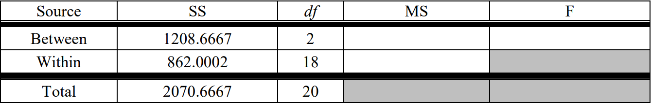.png?revision=1)
Compute the mean squares by dividing the sum of squares by their corresponding \(df\), then add these numbers to the table. \(MSB = \frac{SSB}{k-1} = \frac{1208.66667}{2} = 604.3333 \quad MSW = \frac{SSW}{N-k} = \frac{862}{18} = 47.8889\)
The test statistic is the ratio of these two mean squares: \(F = \frac{MSB}{MSW} = \frac{604.3333}{47.8889} = 12.6195\). Add the test statistic to the table under F.
.png?revision=1)
All ANOVA tests are right-tailed tests, so the critical value for a right-tailed F-test is found with the F-distribution. Use \(\alpha\) = 0.01 area in the right-tail. The degrees of freedom are \(df_{N} = 2\), and \(df_{D} = 18\). The critical value is 6.0129; see the sampling distribution curve in Figure 11-2.
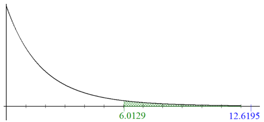.png?revision=1)
Note that the F-distribution starts at zero, and is skewed to the right. The test statistic of 12.6295 is larger than the critical value of 6.0129 so the decision would be to reject the null hypothesis.
Decision: Reject \(H_{0}\).
Summary: There is enough evidence to support the claim that there is a difference in the average age of assistant professors, associate professors, and full professors at her university.
If we were using the p-value method, then we would use the calculator or computer for a right-tailed test. The p-value = 0.0003755 is less than \(\alpha\) = 0.01, which leads to the same decision of rejecting \(H_{0}\) that we found using the critical value method.
.png?revision=1)
Alternatively, use technology to compute the ANOVA table and p-value.
TI-84: ANOVA, hypothesis test for the equality of k population means. Note you have to have the actual raw data to do this test on the calculator. Press the [STAT] key and then the [EDIT] function, type the three lists of data into list one, two and three. Press the [STAT] key, arrow over to the [TESTS] menu, arrow down to the option [F:ANOVA(] and press the [ENTER] key. This brings you back to the regular screen where you should now see ANOVA(. Now hit the [2nd] [L1] [,] [2nd] [L2] [,][2nd] [L3][)] keys in that order. You should now see ANOVA(L1,L2,L3); if you had 4 lists you would then have an additional list.
.png?revision=1)
Press the [ENTER] key. The calculator returns the F-test statistic, the p-value, Factor (Between) \(df\), SS and MS, Error (Within) \(df\), SS and MS. The last value, Sxp is the square root of the MSE.
.png?revision=1)
TI-89: ANOVA, hypothesis test for the equality of \(k\) population means. Go to the [Apps] Stat/List Editor, then type in the data for each group into a separate list (or if you don’t have the raw data, enter the sample size, sample mean and sample variance for group 1 into list1 in that order, repeat for list2, etc.). Press [2nd] then F6 [Tests], then select C:ANOVA. Select the input method data or stats. Select the number of groups. Press the [ENTER] key to calculate. The calculator returns the F-test statistic, the p-value, Factor (Between) df, SS and MS, Error (Within) df, SS and MS. The last value, Sxp, is the square root of the MSE.
.png?revision=1)
Excel: Type the labels and data into adjacent columns (it is important not to have any blank columns, which would be an additional group counted as zeros). Select the Data tab, then Data Analysis, ANOVA: Single-Factor, then OK.
.png?revision=1)
Next, select all three columns of data at once for the input range. Check the box that says Labels in first row (only select this if you actually selected the labels in the input range). Change your value of alpha and output range will be one cell reference where you want your output to start, see below.
.png?revision=1)
You get the following output:
.png?revision=1)
Excel gives both the p-value and critical value so you can use either method when making your decision, but make sure you are comfortable with both.
Summary
The ANOVA test gives evidence that there is a difference between three or more means. The null hypothesis will always have the means equal to one another versus the alternative hypothesis that at least one mean is different. The F-test results are about the difference in means, but the test is actually testing if the variation between the groups is larger than the variation within the groups. If this between group variation is significantly larger than the within groups then we can say there is a statistically significant difference in the population means. Hence, we are always performing a right-tailed F-test for ANOVA. Make sure to only compare the p-value with \(\alpha\) and the test statistic to the critical value.