10.2: Goodness of Fit Test

The \(\chi^{2}\) goodness-of-fit test can be used to test the distribution of three or more proportions within a single population.

Definition: \(\chi^{2}\) goodness-of-fit test

The \(\chi^{2}\)-test is a statistical test for testing the goodness-of-fit of a variable. It can be used when the data are obtained from a random sample and when the expected frequency (E) from each category is 5 or more.

The formula for the \(\chi^{2}\) -test statistic is:

\[\chi^{2}=\sum \frac{(o-E)^{2}}{E}\]

Use a right-tailed \(\chi^{2}\) -distribution with \(\text{df} = k-1\) where \(k\) = the number of categories.

with

• \(O\) = the observed frequency (what was observed in the sample) and
• \(E\) = the expected frequency (based on \(H_{0}\) and the sample size).
• \(H_{0}: p_{1} = p_{0}, p_{2} = p_{0}, \cdots, p_{k} = p_{0}\)
• \(H_{1}:\) At least one proportion is different.

An instructor claims that their students’ grade distribution is different than the department’s grade distribution. The department’s grades have the following proportion of students who get A’s is 35%, B’s is 23%, C’s is 25%, D’s is 10% and F’s is 7% in introductory statistics courses. For a sample of 250 introductory statistics students with this instructor, there were 80 A’s, 50 B’s, 58 C’s, 38 D’s, and 24 F’s. Test the instructor’s claim at the 5% level of significance.

Solution

This is a test for three or more proportions within a single population, so use the goodness-of-fit test. We will always use a right-tailed χ 2 -test. The hypotheses for this example would be:

\(H_{0}: p_{A} = 0.35, p_{B} = 0.23, p_{C} = 0.25, p_{D} = 0.10, p_{F} = 0.07\)

\(H_{1}:\) At least one proportion is different.

Even though there is an inequality in \(H_{1}\), the goodness-of-fit test is always a right-tailed test. This is because we are testing to see if there is a large variation between the observed versus the expected values. If the variance between the observed and expected values is large, then there is a difference in the proportions.

Also note that we do not write the alternative hypothesis as \(p_{A} \neq 0.35, p_{B} \neq 0.23, p_{C} \neq 0.25, p_{D} \neq 0.10, p_{F} \neq 0.07\) since it could be that any one of these proportions is different. All of the proportions not being equal to their hypothesized values is just one possible case.

There are \(k = 5\) categories that we are comparing: A’s, B’s, C’s, D’s and F’s.

The observed counts are the actual number of A’s, B’s, C’s, D’s and F’s from the sample.

We must compute the expected count for each of the five categories. Find the expected counts by multiplying the expected proportion of A’s, B’s, C’s, D’s and F’s by the sample size.

It will be helpful to make a table to organize the work.

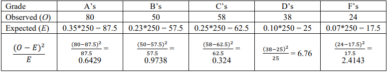
The test statistic is the sum of this last row: \(\chi^{2}=\sum \frac{(O-E)^{2}}{E}=0.6429+0.9783+0.324+6.76+2.4143=11.1195\)

The critical value for a right-tailed \(\chi^{2}\)-test with \(\text{df} = k - 1 = 5 - 1 = 4\) is found by finding the area in the \(\chi^{2}\) -distribution using your calculator or Excel. Use \(\alpha = 0.05\) area in the right-tail, to get the critical value of \(\chi_{\alpha}^{2}\) =CHISQ.INV.RT(0.05,4) = 9.4877. Draw and label the curve as shown in Figure 10-4.

Figure 10-4: Values of \(\chi_{\alpha}^{2}\) and \(\chi^{2}\) on a \(\chi^{2}\)-test with \(\text{df}=4\) and \(\alpha=0.05\).

The test statistic of \(\chi^{2} = 11.1195 > \chi_{\alpha}^{2} = 9.4877\) and is in the rejection area, so our decision is: Reject \(H_{0}\).

There is sufficient evidence to support the claim that the proportion of students who get A’s, B’s, C’s, D’s and F’s in introductory statistics courses for this instructor is different than the department’s proportions of 35%, 23%, 25%, 10% and 7% respectively.

If we were asked to find the p-value, you would just find the area to right of the test statistic (always a right-tailed test) using your calculator or Excel =CHISQ.DIST.RT(11.1195,4) = 0.0253.

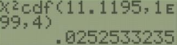
This gives a p-value = 0.0252 which is less than \(\alpha = 0.05\), therefore reject \(H_{0}\).

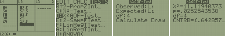
You can use the GOF shortcut function on your calculator to get a p-value; see directions below. If you get the program from your instructor or the website for your TI-83, you can also have the calculator find the \(\frac{(O-E)^{2}}{E}\) values. The TI-84 and 89 already does this.

TI-84: Note: For the TI-83 download a GOF program from http://MostlyHarmlessStatistics.com. Only newer TI-84 operating systems have a calculator shortcut key for GOF. Use the same GOF program as for the TI-83 if your 84 does not have the \(\chi^{2}\) GOF-Test.

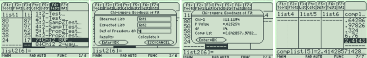
Before you start, write down your observed and expected values. Select Stat, then Calc. Type in the observed values into list 1, and the expected values into list 2. Select Stat, then Tests. Go down to option D: \(\chi^{2}\) GOF-Test. Choose L₁ for the Observed category and L₂ for the Expected category, type in your degrees of freedom (\(\text{df} = k-1\)), and then select Calculate. The calculator returns the \(\chi^{2}\) -test statistic and the p-value. Use the right arrow to see the rest of the \(\frac{(O-E)^{2}}{E}\) values.

TI-89: Go to the [Apps] Stat/List Editor, then type in the observed values into list 1, and the expected values into list 2. Press [2^nd] then F6 [Tests], then select 7: Chi-2GOF. Type in the list names and the degrees of freedom (\(\text{df} = k-1\)). Then press the [ENTER] key to calculate. The calculator returns the \(\chi^{2}\)-test statistic and the p-value. The \(\frac{(O-E)^{2}}{E}\) values are stored in the comp list.

A research company is looking to see if the proportion of consumers who purchase a cereal is different based on shelf placement. They have four locations: Bottom Shelf, Middle Shelf, Top Shelf, and Aisle End Shelf. Test to see whether there is a preference among the four shelf placements. Use the p-value method with \(\alpha=0.05\).

Solution

The hypotheses can be written as a sentence or as proportions. If you use proportions, note that there are no percentages given. We would expect that each shelf placement be the same if there was no preference. There are 4 categories, so \(p_{0} = \frac{1}{4} = 0.25\) or 25% for each placement.

• \(H_{0}: p_{B} = 0.25, p_{M} = 0.25, p_{T} = 0.25, p_{E} = 0.25\)
• \(H_{1}:\) At least one proportion is different.

It is also acceptable to write the hypotheses as a sentence.

• \(H_{0}:\) Proportion of cereal sales is equally distributed across the four shelf placements.
• \(H_{1}:\) Proportion of cereal sales is not equally distributed across the four shelf placements.

Find the expected values. Total all the observed values to get the sample size: \(n = 45 + 67 + 55 + 73 = 240\). Then take the sample size and divide by 4 to get \(\frac{240}{4} = 60\). The expected value for each group is 60.

Compute the test statistic:

\[\begin{aligned} \chi^{2} &=\sum \frac{(O-E)^{2}}{E} = \frac{(45-60)^{2}}{60} + \frac{(67-60)^{2}}{60} + \frac{(55-60)^{2}}{60} + \frac{(73-60)^{2}}{60} \\[4pt] &=3.75+0.816667+0.416667+2.816667=7.8 \end{aligned}\]

Check your work using technology and find the p-value. The degrees of freedom are the number of groups minus one: \(\text{df} = k - 1 = 3\).

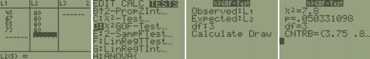
You can scroll right by selecting the right arrow button to see the rest of the contribution values.

In Excel the p-value is found by the formula =CHISQ.DIST.RT(7.8,3). On the TI-Calculator, use the \(\chi^{2}\) GOF-Test shortcut. The p-value = 0.05033 which is larger than \(\alpha=0.05\); therefore, do not reject \(H_{0}\).

There is not enough evidence to support the claim that cereal shelf placement makes a statistically significant difference in the proportion of sales at the 5% level of significance.