9.6: Chapter 9 Formulas

Hypothesis Test for 2 Dependent Means \(\mathrm{H}_{0}: \mu_{\mathrm{D}}=0\) \(\mathrm{H}_{1}: \mu_{\mathrm{D}} \neq 0\) \(t=\frac{\bar{D}-\mu_{D}}{\left(\frac{S_{D}}{\sqrt{n}}\right)}\) TI-84: T-Test	Confidence Interval for 2 Dependent Means \(\bar{D} \pm t_{\alpha / 2}\left(\frac{s_{D}}{\sqrt{n}}\right)\) TI-84: TInterval
Hypothesis Test for 2 Independent Means Z-Test: \(\begin{aligned} \mathrm{H}_{0}: \mu_{1} &=\mu_{2} \\ \mathrm{H}_{1}: \mu_{1} & \neq \mu_{2} \end{aligned}\) \(z=\frac{\left(\bar{x}_{1}-\bar{x}_{2}\right)-\left(\mu_{1}-\mu_{2}\right)_{0}}{\sqrt{\left(\frac{\sigma_{1}^{2}}{n_{1}}+\frac{\sigma_{2}^{2}}{n_{2}}\right)}}\) TI-84: 2-SampZTest	Confidence Interval for 2 Independent Means Z-Interval \(\left(\bar{x}_{1}-\bar{x}_{2}\right) \pm z_{\alpha / 2} \sqrt{\left(\frac{\sigma_{1}^{2}}{n_{1}}+\frac{\sigma_{2}^{2}}{n_{2}}\right)} \) TI-84: 2-SampZInt
Hypothesis Test for 2 Independent Means \(\begin{aligned} &\mathrm{H}_{0}: \mu_{1}=\mu_{2} \\ &\mathrm{H}_{1}: \mu_{1} \neq \mu_{2} \end{aligned}\) T-Test: Assume variances are unequal \(t=\frac{\left(\bar{x}_{1}-\bar{x}_{2}\right)-\left(\mu_{1}-\mu_{2}\right)_{0}}{\sqrt{\left(\frac{s_{1}^{2}}{n_{1}}+\frac{s_{2}^{2}}{n_{2}}\right)}}\) TI-84: 2-SampTTest \(df=\frac{\left(\frac{s_{1}^{2}}{n_{1}}+\frac{s_{2}^{2}}{n_{2}}\right)^{2}}{\left(\left(\frac{s_{1}^{2}}{n_{1}}\right)^{2}\left(\frac{1}{n_{1}-1}\right)+\left(\frac{s_{2}^{2}}{n_{2}}\right)^{2}\left(\frac{1}{n_{2}-1}\right)\right)}\) T-Test: Assume variances are equal \(\begin{aligned} &t=\frac{\left(\bar{x}_{1}-\bar{x}_{2}\right)-\left(\mu_{1}-\mu_{2}\right)}{\sqrt{\left(\frac{\left(n_{1}-1\right) s_{1}^{2}+\left(n_{2}-1\right) s_{2}^{2}}{\left(n_{1}+n_{2}-2\right)}\right)\left(\frac{1}{n_{1}}+\frac{1}{n_{2}}\right)}} \\ &d f=\mathrm{n}_{1}-\mathrm{n}_{2}-2 \end{aligned}\)	Confidence Interval for 2 Independent Means \(\left(\bar{x}_{1}-\bar{x}_{2}\right) \pm t_{\alpha / 2} \sqrt{\left(\frac{s_{1}^{2}}{n_{1}}+\frac{s_{2}^{2}}{n_{2}}\right)}\) TI-84: 2-SampTInt \(df=\frac{\left(\frac{s_{1}^{2}}{n_{1}}+\frac{s_{2}^{2}}{n_{2}}\right)^{2}}{\left(\left(\frac{s_{1}^{2}}{n_{1}}\right)^{2}\left(\frac{1}{n_{1}-1}\right)+\left(\frac{s_{2}^{2}}{n_{2}}\right)^{2}\left(\frac{1}{n_{2}-1}\right)\right)}\) T-Interval: Assume variances are equal \(\begin{aligned} &\left(\bar{x}_{1}-\bar{x}_{2}\right) \pm t_{\alpha / 2} \sqrt{\left(\left(\frac{\left(n_{1}-1\right) s_{1}^{2}+\left(n_{2}-1\right) s_{2}^{2}}{\left(n_{1}+n_{2}-2\right)}\right)\left(\frac{1}{n_{1}}+\frac{1}{n_{2}}\right)\right)} \\ &d f=\mathrm{n}_{1}-\mathrm{n}_{2}-2 \end{aligned}\)
Hypothesis Test for 2 Proportions \(\begin{aligned} &\mathrm{H}_{0}: p_{1}=p_{2} \\ &\mathrm{H}_{1}: p_{1} \neq p_{2} \end{aligned}\) \(Z=\frac{\left(\hat{p}_{1}-\hat{p}_{2}\right)-\left(p_{1}-p_{2}\right)}{\sqrt{\left(\hat{p} \cdot \hat{q}\left(\frac{1}{n_{1}}+\frac{1}{n_{2}}\right)\right)}}\) \(\hat{p}=\frac{\left(x_{1}+x_{2}\right)}{\left(n_{1}+n_{2}\right)}=\frac{\left(\hat{p}_{1} \cdot n_{1}+\hat{p}_{2} \cdot n_{2}\right)}{\left(n_{1}+n_{2}\right)}\) \(\hat{q}=1-\hat{p} \quad \hat{p}_{1}=\frac{x_{1}}{n_{1}} \hat{p}_{2}=\frac{x_{2}}{n_{2}}\) TI-84: 2-PropZInt	Confidence Interval for 2 Proportions \(\left(\hat{p}_{1}-\hat{p}_{2}\right) \pm z_{\frac{\alpha}{2}} \sqrt{\left(\frac{\hat{p}_{1} \hat{q}_{1}}{n_{1}}+\frac{\hat{p}_{2} \hat{q}_{2}}{n_{2}}\right)}\) \(\hat{p}_{1}=\frac{x_{1}}{n_{1}} \quad \hat{p}_{2}=\frac{x_{2}}{n_{2}}\) \(\hat{q}_{1}=1-\hat{p}_{1} \quad \hat{q}_{2}=1-\hat{p}_{2}\) TI-84: 2-PropZInt
Hypothesis Test for 2 Variances \(\begin{aligned} &H_{0}: \sigma_{1}^{2}=\sigma_{2}^{2} \\ &H_{1}: \sigma_{1}^{2} \neq \sigma_{2}^{2} \end{aligned} \quad F=\frac{s_{1}^{2}}{s_{2}^{2}}\) \(df \mathrm{~N}=\mathrm{n}_{1}-1, df \mathrm{D}=\mathrm{n}_{2}-1\) TI-84: 2-SampFTest	Hypothesis Test for 2 Standard Deviations \(\begin{aligned} &H_{0}: \sigma_{1}=\sigma_{2} \\ &H_{1}: \sigma_{1} \neq \sigma_{2} \end{aligned} \quad F=\frac{s_{1}^{2}}{s_{2}^{2}}\) \(df \mathrm{~N}=\mathrm{n}_{1}-1, df \mathrm{D}=\mathrm{n}_{2}-1\) TI-84: 2-SampFTest

The following flow chart in Figure 9-18 can help you decide which formula to use. Start on the left, ask yourself is the question about proportions (%), means (averages), standard deviations or variances? Are there 1 or 2 samples? Was the population standard deviation given? Are the samples dependent or independent? Are you asked to test a claim? If yes then use the test statistic (TS) formula. Are you asked to find a confidence interval? If yes then use the confidence interval (CI) formula. In each box is the null hypothesis and the corresponding TI calculator shortcut key.

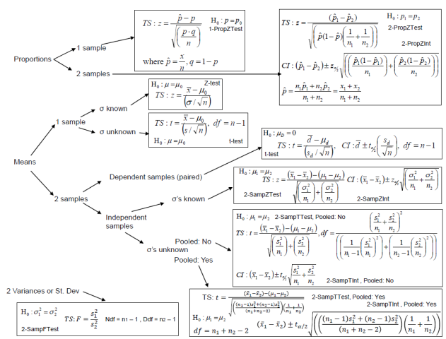
Figure 9-18

Download a .pdf version of the flowchart at: http://MostlyHarmlessStatistics.com.

The same steps are used in hypothesis testing for a one sample test. Use technology to find the p-value or critical value. A clue with many of these questions of whether the samples are dependent is the term “paired” is used, or the same person was being measured before and after some applied experiment or treatment. The p-value will always be a positive number between 0 and 1.

The same three methods to hypothesis testing, critical value method, p-value method and the confidence interval method are also used in this section. The p-value method is used more often than the other methods. The rejection rule for the three methods are:

• P-value method: reject H₀ when the p-value ≤ \(\alpha\).
• Critical value method: reject H₀ when the test statistic is in the critical tail(s).
• Confidence Interval method, reject H₀ when the hypothesized value (0) found in H₀ is outside the bounds of the confidence interval.

The most important step in any method you use is setting up your null and alternative hypotheses.