9.2: Two Independent Groups

This section will look at how to analyze a difference in the mean for two independent samples. As with all other hypothesis tests and confidence intervals, the process is the same, though the formulas and assumptions are different.

The symbol used for the population mean has been \(μ\) up to this point. In order to use formulas that compare the means from two populations, we use subscripts to show which population statistic or parameter we are referencing.

Parameters

• µ₁ = population mean of population 1
• µ₂ = population mean of population 2
• σ₁ = population standard deviation of population 1
• σ₂ = population standard deviation of population 2
• \(\sigma_{1}^{2}\) = population variance of population 1
• \(\sigma_{1}^{2}\) = population variance of population 2
• p₁ = population proportion of population 1
• p₂ = population proportion of population 2

Statistics

• \(\bar{x}_{1}\) = mean of sample from population 1
• \(\bar{x}_{2}\) = mean of sample from population 2
• s₁ = standard deviation of sample from population 1
• s₂ = standard deviation of sample from population 2
• \(s_{1}^{2}\) = variance of sample from population 1
• \(s_{2}^{2}\) = variance of sample from population 2
• \(\hat{p}_{1}\) = proportion of sample from population 1
• \(\hat{p}_{2}\) = proportion of sample from population 2
• n₁ = sample size from population 1
• n₂ = sample size from population 2

You do not need to use the subscripts 1 and 2. You can use a letter or symbol that helps you differentiate between the two groups. For instance, if you have two manufacturers labeled A and B, you may want to use µ_A and µ_B.

When setting up the null hypothesis we are testing if there is a difference in the two means equal to some known difference. H₀: µ₁ – µ₂ = (µ₁ – µ₂)₀. We will focus on the case where (µ₁ – µ₂)₀ = 0, which says that, tentatively, we assume that there is no difference in population means H₀: µ₁ – µ₂ = 0. If we were to subtract μ₂ from both sides of the equation µ₁ – µ₂ = 0 we would get µ₁ = µ₂. For instance, if the average age for group one was 25 and the average age for group two was also 25, then the difference between the two means would be 25 – 25 = 0.

There are three ways to set up the hypotheses for comparing two independent population means µ₁ and µ₂.

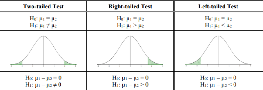
Figure 9-3

For a one-tailed test, one could alternatively write the null hypotheses as:

Right-tailed test Left-tailed test

H₀: µ₁ ≤ µ₂ H₀: µ₁ ≥ µ₂

H₁: µ1 > µ₂ H₁: µ₁ < µ₂

This text mostly will use an = sign in the null hypothesis.

Most of the time the groups are numbered from the order in which their statistics or data appear in the problem. To keep the correct sign of the test, make sure you do not switch the order of the groups.

For instance, if we were comparing the mean SAT score between high school juniors and seniors and our hypothesis is that the mean for seniors is higher we could set up the alternative hypotheses as either µ_j < µ_s if we had the juniors be group 1 and µ_j > µ_s if we had the seniors be group 1. This change would switch the sign of both the test statistic and the critical value.

When performing a one-tailed test the sign of the test statistic and critical value will match most of the time. For example, if your test statistic came out to be z = –1.567 and your critical value was z = 1.645 you most likely have the incorrect order in your hypotheses.

When you are making a conjecture about a population mean, we have two different situations, depending on if we know that population standard deviation, or not, called the z-test and t-test, respectively. Use Figure 9-4 to help decide when to use the z-test and t-test.

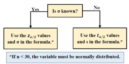
Figure 9-4

Note that you should never use the value of σ_x on your calculator since you would rarely ever have an entire population of raw data to input into a calculator. The problem may give you raw data, but σ or σ2 would be stated in the problem and you should be using a z-test, otherwise use the t-test with the sample standard deviation s_x. Usually, σ is known from a previous year or similar study.

In either case if the sample sizes are below 30 we need to check that the population is approximately normally distributed for the Central Limit Theorem to hold. We can do this with a normal probability plot. Most examples that we deal with just assume the population is normally distributed, but in practice, you should always check these assumptions.

9.3.1 Two Sample Mean Z-Test & Confidence Interval

The two-sample z-test is a statistical test for comparing the means from two independent populations with σ1 and σ2 stated in the problem and using the formula for the test statistic

\(z=\frac{\left(\bar{x}_{1}-\bar{x}_{2}\right)-\left(\mu_{1}-\mu_{2}\right)}{\sqrt{\left(\frac{\sigma_{1}^{2}}{n_{1}}+\frac{\sigma_{2}^{2}}{n_{2}}\right)}}\)

Note that µ₁ – µ₂ is the hypothesized difference found in the null hypothesis and is usually zero.

The traditional method (or critical value method), the p-value method, and the confidence interval method are performed with steps that are identical to those when performing hypothesis tests for one population. We will show an example of a two-sample z-test, but seldom in practice will we perform this type of test since we rarely have access to a population standard deviation.

A university adviser wants to see whether there is a significant difference in ages of full-time students and part-time students. They select a random sample of 50 students from each group. The ages are shown below. At \(\alpha\) = 0.05, decide if there is enough evidence to support the claim that there is a difference in the ages of the two groups. Assume the population standard deviation for full-time students is 3.68 years old and for part-time students is 4.7 years old. Use the p-value method.

Full-time students

22 25 27 23 26 28 26 24 25 20 19 18 30 26 18 18 19 32 23 19 18 22 26 19 19 21 23 18 20 18 22 18 20 19 23 26 24 27 26 18 22 21 19 21 21 19 18 29 19 22

Part-time students

18	20	19	18	22	25	24	35	23	18
24	26	30	22	22	22	21	18	20	19
19	32	29	23	21	19	36	27	27	20
20	19	19	20	25	23	22	28	25	20
20	21	18	19	23	26	35	19	19	18

Solution

Assumptions: The two populations we are sampling from are not necessarily normal, but the sample sizes are greater than 30, so the Central Limit Theorem holds. The population standard deviations σ₁ and σ₂ are known; therefore, we use the z-test for comparing two population means µ₁ and µ₂.

The claim is that there is a difference in the ages of the two student groups. Let full-time students be population 1 and part-time students be population 2 (always go in the same order as the data are presented in the problem unless otherwise stated). Then µ₁ would be the average age for full-time students and µ₂ would be the average age for parttime students. The key phrase is difference: µ₁ ≠ µ₂.

The correct hypotheses are H₀: µ₁ = µ₂

H₁: µ₁ ≠ µ₂.

This is a two-tailed test and the claim is in the alternative hypothesis.

Note that if we had decided to have population 1 be part-time students, the test statistic would be negated from that given below, but the p-value and result would be identical. In general, you should take population 1 as whatever group comes first in the problem.

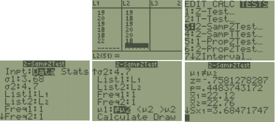
Using technology, we compute \(\bar{x}_{1}\) = 22.12, \(\bar{x}_{2}\) = 22.76, n₁ = 50 and n₂ = 50. From the problem we have σ₁ = 3.68 and σ₂ = 4.7. Since µ₁ = µ₂ then we know that µ₁ – µ₂ = 0, and that we do not use the sample standard deviations.

The test statistic is: \(Z=\frac{\left(\bar{x}_{1}-\bar{x}_{2}\right)-\left(\mu_{1}-\mu_{2}\right)_{0}}{\sqrt{\left(\frac{\sigma_{1}^{2}}{n_{1}}+\frac{\sigma_{2}^{2}}{n_{2}}\right)}}=\frac{(22.12-22.76)-0}{\sqrt{\left(\frac{3.68^{2}}{50}+\frac{4.7^{2}}{50}\right)}}=-0.7581\).

The p-value for a two-tailed z-test is found by finding the area to the left (since z is negative) of the test statistic using a normal distribution and multiplying the area by two. Using the normalcdf(–∞,–0.7581, 0,1) we get an area of 0.2242. Since this is a two-tailed test we need to double the area, which gives a p-value = 0.4484.

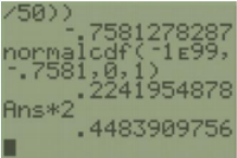
Note that if the z-score was positive, find the area to the right of z, then double.

Decision: Because the p-value = 0.4484 is larger than \(\alpha\) = 0.05, we do not reject H₀.

Summary: At the 5% level of significance, there is not enough evidence to support the claim that there is a difference in the ages of full-time students and part-time students.

TI-84: Press the [STAT] key, arrow over to the [TESTS] menu, arrow down to the option [3:2-SampZTest] and press the [ENTER] key. Arrow over to the [Data] menu and press the [ENTER] key. Then type in the population standard deviations, the first sample mean and sample size, then the second sample mean and sample size, arrow over to the \(\neq\), <, > sign that is the same in the problem’s alternative hypothesis statement, then press the [ENTER]key, arrow down to [Calculate] and press the [ENTER] key. The calculator returns the test statistic z and the p-value.

TI-89: Go to the [Apps] Stat/List Editor, then press [2^nd] then F6 [Tests], then select 3: 2-SampZ-Test. Then type in the population standard deviations, the first sample mean and sample size, then the second sample mean and sample size (or list names (list3 & list4), and Freq1:1 & Freq2:1), arrow over to the \(\neq\), <, > sign that is the same in the problem’s alternative hypothesis statement then press the [ENTER] key to calculate. The calculator returns the z-test statistic and the p-value.

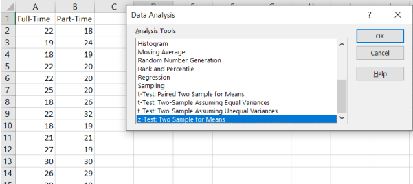
Excel: Start by entering the data in two columns in the same order that they appear in the problem. Then select Data > Data Analysis > z-test: Two Sample for Means, then select OK.

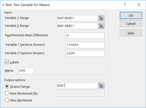
Click into the box next to Variable 1 Range and select the cells where the first data set is, including the label. Click into the box next to Variable 2 Range and select the cells where the second data set is, including the label. Type in zero for the hypothesized mean; this comes from the null hypothesis that if µ₁ = µ₂ then µ₁ – µ₂ = 0.

Type in the variance for each group, and be careful with this step: the variance is the standard deviation squared \(\sigma_{1}^{2}\) = 3.68² = 13.5424 and \(\sigma_{2}^{2}\) = 4.7² = 22.09. Select the Label box only if you highlighted the label in the variable range box. Change alpha to fit the significance level given in the problem. The output range is one cell reference number where you want the top left-hand corner of your output table to start, or you can use the default to have your output open in a new worksheet. Then select Ok. See Excel output below.

You get the following output in Excel:

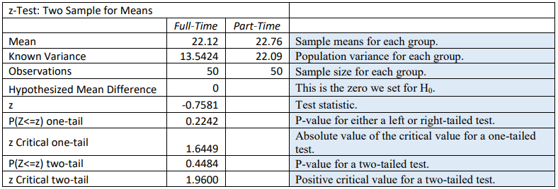
Note you can only use the Excel shortcut if you have the raw data. If you have summarized data then you would need to do everything by hand.

Two-Sample Z-Interval

For independent samples, we take the mean of each sample, then take the difference in the means. If the means are equal, then the difference of the two means would be equal to zero. We can then compare the null hypothesis, that there is no difference in the means μ₁ – μ₂ = 0, with the confidence interval limits to decide whether to reject the null hypothesis. If zero is contained within the confidence interval, then we fail to reject H₀. If zero is not contained within the confidence interval, then we reject H₀.

A (1 – \(\alpha\))*100% confidence interval for the difference between two population means µ₁ – µ₂ :

\(\left(\bar{x}_{1}-\bar{x}_{2}\right) \pm z_{\alpha / 2} \sqrt{\left(\frac{\sigma_{1}^{2}}{n_{1}}+\frac{\sigma_{2}^{2}}{n_{2}}\right)}\)

The requirements for the confidence interval are identical to the previous hypothesis test.

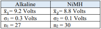
Non-rechargeable alkaline batteries and nickel metal hydride (NiMH) batteries are tested, and their voltage is compared. The data follow. Test to see if there is a difference in the means using a 95% confidence interval. Assume that both variables are normally distributed.

Solution

First, set up the hypotheses H₀: µ₁ = µ₂

H₁: µ₁ ≠ µ₂.

Next, find the \(z_{\alpha / 2}\) critical value for a 95% confidence interval. Use technology to get \(z_{\alpha / 2}\) = 1.96.

Find the interval estimate (confidence interval): \(\left(\bar{x}_{1}-\bar{x}_{2}\right) \pm z_{\alpha / 2} \sqrt{\left(\frac{\sigma_{1}^{2}}{n_{1}}+\frac{\sigma_{2}^{2}}{n_{2}}\right)}\)

\(\begin{aligned}
&\Rightarrow(9.2-8.8) \pm 1.96 \sqrt{\left(\frac{0.3^{2}}{27}+\frac{0.1^{2}}{30}\right)} \\
&\Rightarrow \quad 0.4 \pm 0.1187 .
\end{aligned}\)

Use interval notation (0.2813, 0.5187) or standard notation 0.28 < µ₁ – µ₂ < 0.52.

For an interpretation, if we were to use the same sampling techniques, approximately 95 out of 100 times the confidence interval (0.2813, 0.5187) would contain the population mean difference in voltage between alkaline and NiMH batteries. Since both endpoints are positive, we can reject H₀. We can be 95% confident that the population mean voltage for alkaline batteries is between 0.28 and 0.52 volts higher than nickel metal hydride batteries.

There is no shortcut option for a two-sample z confidence interval in Excel.

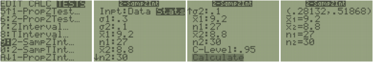
TI-84: Press the [STAT] key, arrow over to the [TESTS] menu, arrow down to the option [9:2-SampZInt] and press the [ENTER] key. Arrow over to the [Stats] menu and press the [ENTER] key. Then type in the population standard deviations, the first sample mean and sample size, then the second sample mean and sample size, then enter the confidence level. Arrow down to [Calculate] and press the [ENTER] key. The calculator returns the confidence interval.

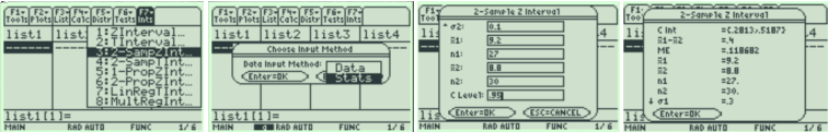
TI-89: Go to the [Apps] Stat/List Editor, then press [2^nd] then F5 [Ints], then select 3: 2-SampZInt. Then type in the population standard deviations, the first sample mean and sample size, then the second sample mean and sample size (or list names (list3 & list4), and Freq1:1 & Freq2:1), then enter the confidence level. To calculate press the [ENTER] key. The calculator returns the confidence interval.

9.3.2 Two Sample Mean T-Test & Confidence Interval

The t-test is a statistical test for comparing the means from two independent populations. The t-test is used when σ₁ and/or σ₂ are both unknown. The samples must be independent and if the sample sizes are less than 30 then the populations need to be normally distributed. The t-test, as opposed to the z-test, for two independent samples has two different versions depending on if a particular assumption that the unknown population variances are unequal or equal. Since we do not know the true value of the population variances, we usually will use the first version and assume that the population variances are not equal \(\sigma_{1}^{2} \neq \sigma_{2}^{2}\). Both versions are presented, so make sure to check with your instructor if you are using both versions.

9.3.2.a Unequal Variance Method t-Test

If we assume the variances are unequal (\(\sigma_{1}^{2} \neq \sigma_{2}^{2}\)), the formula for the t test statistic is

\(t=\frac{\left(\bar{x}_{1}-\bar{x}_{2}\right)-\left(\mu_{1}-\mu_{2}\right)}{\sqrt{\left(\frac{s_{1}^{2}}{n_{1}}+\frac{s_{2}^{2}}{n_{2}}\right)}}\)

Use the t-distribution where the degrees of freedom are \(d f=\frac{\left(\frac{s_{1}^{2}}{n_{1}}+\frac{s_{2}^{2}}{n_{2}}\right)^{2}}{\left(\left(\frac{s_{1}^{2}}{n_{1}}\right)^{2}\left(\frac{1}{n_{1}-1}\right)+\left(\frac{s_{2}^{2}}{n_{2}}\right)^{2}\left(\frac{1}{n_{2}-1}\right)\right)}\).

Note that µ₁ – µ₂ is the hypothesized difference found in the null hypothesis and is usually zero.

Some older calculators only accept the df as an integer, in this case round the df down to the nearest integer if needed. For most technology, you would want to keep the decimal df.

Some textbooks use an approximation for the df as the smaller of n₁ – 1 or n₂ – 1, so you may find a different answer using your calculator compared to examples found elsewhere.

The traditional method (or critical value method), the p-value method, and the confidence interval method are performed with steps that are identical to those when performing hypothesis tests for one population.

The sample sizes both need to be 30 or more, or the populations need to be approximately normally distributed in order for the Central Limit Theorem to hold.

Two-Sample T-Interval

For independent samples, we take the mean of each sample, then take the difference in the means. If the means are equal, then the difference of the two means would be equal to zero. We can then compare the null hypothesis, that there is no difference in the means μ₁ – μ₂ = 0, with the confidence interval limits to decide whether to reject the null hypothesis. If zero is contained within the confidence interval, then we fail to reject H₀. If zero is not contained within the confidence interval, then we reject H_0.

A (1 – \(\alpha\))*100% confidence interval for the difference between two population means μ₁ – μ₂ for independent samples with unequal variances: \(\left(\bar{x}_{1}-\bar{x}_{2}\right) \pm t_{\alpha / 2} \sqrt{\left(\frac{s_{1}^{2}}{n_{1}}+\frac{s_{2}^{2}}{n_{2}}\right)}\).

The requirements and degrees of freedom are identical to the above hypothesis test.

The general United States adult population volunteer an average of 4.2 hours per week. A random sample of 18 undergraduate college students and 20 graduate college students indicated the results below concerning the amount of time spent in volunteer service per week. At \(\alpha\) = 0.01 level of significance, is there sufficient evidence to conclude that a difference exists between the mean number of volunteer hours per week for undergraduate and graduate college students? Assume that number of volunteer hours per week is normally distributed.

  UndergraduateGraduate Sample Mean 2.5 3.8 Sample Variance 2.2 3.5 Sample Size 18 20

Solution

Assumptions: The two populations we are comparing are undergraduate and graduate college students. We are given that the number of volunteer hours per week is normally distributed. We are told that the samples were randomly selected and should therefore be independent. We do not know the two population standard deviations (we only have the sample standard deviations as the square root of the sample variances), so we must use the t-test. Using the critical value method steps, we get the following.

The question is asking if there is a difference between the mean number of volunteer hours per week for undergraduate and graduate level college students. We let population 1 be undergraduate students, and population 2 be graduate students.

The correct hypotheses for a two-tailed test are: H₀: µ₁ = µ₂

H₁: µ₁ ≠ µ₂.

The test statistic is \(t=\frac{\left(\bar{x}_{1}-\bar{x}_{2}\right)-\left(\mu_{1}-\mu_{2}\right)}{\sqrt{\left(\frac{s_{1}^{2}}{n_{1}}+\frac{s_{2}^{2}}{n_{2}}\right)}}=\frac{(2.5-3.8)-0}{\sqrt{\left(\frac{2.2}{18}+\frac{3.5}{20}\right)}}=-2.3845\).

The critical value for a two-tailed t-test with degrees of freedom is found by using tail area \(\alpha\)/2 = 0.005 with

\(df=\frac{\left(\frac{s_{1}^{2}}{n_{1}}+\frac{s_{2}^{2}}{n_{2}}\right)^{2}}{\left(\left(\frac{s_{1}^{2}}{n_{1}}\right)^{2}\left(\frac{1}{n_{1}-1}\right)+\left(\frac{s_{2}^{2}}{n_{2}}\right)^{2}\left(\frac{1}{n_{2}-1}\right)\right)}=\frac{\left(\frac{2.2}{18}+\frac{3.5}{20}\right)^{2}}{\left(\left(\frac{2.2}{18}\right)^{2}\left(\frac{1}{17}\right)+\left(\frac{3.5}{20}\right)^{2}\left(\frac{1}{19}\right)\right)}=35.0753\).

Draw the curve and label the critical values. Use the invT function on your calculator to compute the critical value invT(.005,35.0753) = –2.724 (older calculators may require you to use a whole number, round down to df = 35), or use Excel =T.INV(0.005,35.0753) to compute the critical value.

The test statistic is between the critical values –2.724 and 2.724, therefore do not reject H₀.

Figure 9-5

There is not enough evidence to suggest a difference between the population mean number of volunteer hours per week for undergraduate and graduate college students.

Note that if we had decided to have population 1 be graduate students, the test statistic would be positive 2.3845, but this would not change our decision for a two-tailed test. If you are doing a one-tailed test, then you need to be consistent on which sign your test statistic has. Most of the time for a left-tailed test both the critical value and the test statistic will be negative and for a right-tailed test both the critical value and test statistic will be positive.

TI-84: Press the [STAT] key, arrow over to the [TESTS] menu, arrow down to the option [4:2-SampTTest] and press the [ENTER] key. Arrow over to the [Stats] menu and press the [Enter] key. Enter the means, standard deviations, sample sizes, confidence level. Then arrow over to the not equal <, > sign that is the same in the problem’s alternative hypothesis statement, then press the [ENTER] key. Highlight the No option under Pooled for unequal variances. Arrow down to [Calculate] and press the [ENTER] key. The calculator returns the test statistic and the p-value. If you have raw data, press the [STAT] key and then the [EDIT] function, then enter the data into list one and list two. Press the [STAT] key, arrow over to the [TESTS] menu, arrow down to the option [4:2- SampTTest] and press the [ENTER] key. Arrow over to the [Data] menu and press the [ENTER] key. The defaults are List1: L₁, List2: L₂, Freq1:1, Freq2:1. If these are set different arrow down and use [2^nd] [1] to get L₁ and [2^nd] [2] to get L₂.

TI-89: Go to the [Apps] Stat/List Editor, then press [2^nd] then F6 [Tests], then select 4: 2-SampT-Test. Enter the sample means, sample standard deviations, and sample sizes (or list names (list3 & list4), and Freq1:1 & Freq2:1). Then arrow over to the not equal, <, > and select the sign that is the same in the problem’s alternative hypothesis statement. Highlight the No option under Pooled. Press the [ENTER] key to calculate. The calculator returns the t-test statistic and the p-value.

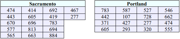
A researcher is studying how much electricity (in kilowatt hours) households from two different cities use in their homes. Random samples of 17 days in Sacramento and 16 days in Portland are given below. Test to see if there is a difference using all 3 methods (critical value, p-value and confidence interval). Assume that electricity use is normally distributed and the population variances are unequal. Use \(\alpha\) = 0.10.

Solution

The populations are independent and normally distributed.

The hypotheses for all 3 methods are: H₀: µ₁ = µ₂

H₁: µ₁ ≠ µ₂.

Use technology to find the sample means, standard deviations and sample sizes.

Enter the Sacramento data into list 1, then do 1-Var Stats L1 and you should get \(\bar{x}_{1}\) = 596.2353, s₁ = 163.2362, and n₁ = 17.

Enter the Portland data into list 2, then do 1-Var Stats L2 and you should get \(\bar{x}_{2}\) = 481.5, s₁ = 179.3957, and n₁ = 16.

The test statistic is \(t=\frac{\left(\bar{x}_{1}-\bar{x}_{2}\right)-\left(\mu_{1}-\mu_{2}\right)_{0}}{\sqrt{\left(\frac{s_{1}^{2}}{n_{1}}+\frac{s_{2}^{2}}{n_{2}}\right)}}=\frac{(596.2353-481.5)-0}{\sqrt{\left(\frac{163.2362^{2}}{17}+\frac{179.3957^{2}}{16}\right)}}=1.9179\).

The \(df=\frac{\left(\frac{s_{1}^{2}}{n_{1}}+\frac{s_{2}^{2}}{n_{2}}\right)^{2}}{\left(\left(\frac{s_{1}^{2}}{n_{1}}\right)^{2}\left(\frac{1}{n_{1}-1}\right)+\left(\frac{s_{2}^{2}}{n_{2}}\right)^{2}\left(\frac{1}{n_{2}-1}\right)\right)}=\frac{\left(\frac{163.2362^{2}}{17}+\frac{179.3957^{2}}{16}\right)^{2}}{\left(\left(\frac{163.266^{2}}{17}\right)^{2}\left(\frac{1}{16}\right)+\left(\frac{179.3957^{2}}{16}\right)^{2}\left(\frac{1}{15}\right)\right)}=30.2598\).

The p-value would be double the area to the right of t = 1.9179. Using the TI calculator or Excel we get the p-value = 0.0646. Stop and see if you can find this p-value using the same process from previous sections.

Since the p-value is less than alpha, we would reject H₀.

At the 10% level of significance, there is a statistically significant difference between the mean electricity use in Sacramento and Portland.

Excel

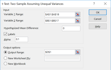
When you have raw data, you can use Excel to find all this information using the Data Analysis tool. Enter the data into Excel, then choose Data > Data Analysis > t-Test: Two Sample Assuming Unequal Variances.

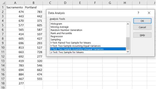
Enter the necessary information as we did in previous sections (see output below) and select OK.

You can use this Excel shortcut only if you have raw data given in the question.

We get the following output, which has both p-values and critical values.

Critical Value Method

The hypotheses and test statistic steps do not change compared to the p-value method.

Hypotheses: H₀: µ₁ = µ₂

H₁: µ₁ ≠ µ₂.

Test Statistic: \(t=\frac{\left(\bar{x}_{1}-\bar{x}_{2}\right)-\left(\mu_{1}-\mu_{2}\right)_{0}}{\sqrt{\left(\frac{s_{1}^{2}}{n_{1}}+\frac{s_{2}^{2}}{n_{2}}\right)}}=\frac{(596.2353-481.5)-0}{\sqrt{\left(\frac{163.2362^{2}}{17}+\frac{179.3957^{2}}{16}\right)}}=1.9179\)

Compute the t critical values.

The degrees of freedom stay the same: \(df=\frac{\left(\frac{163.2362^{2}}{17}+\frac{179.3957^{2}}{16}\right)^{2}}{\left(\left(\frac{163.2362^{2}}{17}\right)^{2}\left(\frac{1}{16}\right)+\left(\frac{179.3957^{2}}{16}\right)^{2}\left(\frac{1}{15}\right)\right)}=30.2598\)

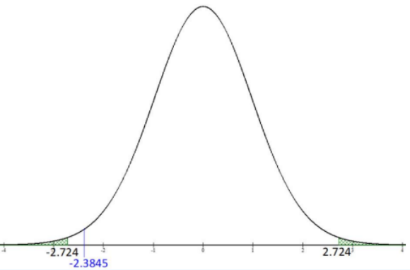
We can use the t Critical two-tail value given in the Excel output or use the TIcalculator invT(0.05,30.2598) = -1.697. Some older calculators do not let you use a decimal for df so round down and use invT(0.05,30).

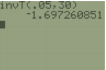
Figure 9-6.

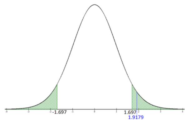
Figure 9-6

Since the test statistic is in the critical region, we would reject H₀. This agrees with the same decision that we had using the p-value method.

Summary: At the 10% level of significance, there is statistically significant difference between the mean electricity use between Sacramento and Portland.

Confidence Interval Method

The hypotheses are the same. The main difference is that we would find a confidence interval and compare H₀: µ₁ – µ₂ = 0 with the endpoints to make the decision.

Hypotheses: H₀: µ₁ = µ₂

H₁: µ₁ ≠ µ₂.

Find the confidence interval. First, compute the \(\mathrm{t}_{\alpha / 2}\) critical value for a 90% confidence interval since \(\alpha\) = 0.10.

Use \(df=\frac{\left(\frac{s_{1}^{2}}{n_{1}}+\frac{s_{2}^{2}}{n_{2}}\right)^{2}}{\left(\left(\frac{s_{1}^{2}}{n_{1}}\right)^{2}\left(\frac{1}{n_{1}-1}\right)+\left(\frac{s_{2}^{2}}{n_{2}}\right)^{2}\left(\frac{1}{n_{2}-1}\right)\right)}=\frac{\left(\frac{163.2362^{2}}{17}+\frac{179.3957^{2}}{16}\right)^{2}}{\left(\left(\frac{163.236^{2}}{17}\right)^{2}\left(\frac{1}{16}\right)+\left(\frac{179.395^{2}}{16}\right)^{2}\left(\frac{1}{15}\right)\right)}=30.2598\).

The critical value is \(\mathrm{t}_{\alpha / 2}\) = invT(0.05,30.2598) = –1.697.

The older TI-83 invT program only accepts integer df, use df =30. Alternatively, use the output from the Excel output under the t Critical two-tail row.

Next, find the interval estimate \(\left(\bar{x}_{1}-\bar{x}_{2}\right) \pm t_{\alpha / 2} \sqrt{\left(\frac{s_{1}^{2}}{n_{1}}+\frac{s_{2}^{2}}{n_{2}}\right)}\)

\(\begin{aligned}
&\Rightarrow(596.2353-481.5) \pm 1.697 \sqrt{\left(\frac{163.2362^{2}}{17}+\frac{179.3957^{2}}{16}\right)} \\
&\Rightarrow \quad 114.7353 \pm 101.5203 .
\end{aligned}\)

Use interval notation (13.215, 216.2556) or standard notation 13.215 < μ₁ – μ₂ < 216.2556. Note the calculator does not round between steps and gives a more accurate answer of (13.23, 216.24).

For an interpretation, if we were to use the same sampling techniques, approximately 90 out of 100 times a confidence interval with the same margin of error of (13.23, 216.24) would contain the population mean difference in electricity use between Sacramento and Portland.

We are 90% confident that the population mean household electricity use for Sacramento is between 13.23 and 216.24 kilowatt hours more than Portland households.

Since both endpoints are positive, zero would not be captured in the confidence interval so we would reject H₀.

Summary: At the 10% level of significance, there is statistically significant difference between the mean electricity use between Sacramento and Portland.

All 3 methods should yield the same result. This text is only using the two-sided confidence interval.

TI-84: Press the [STAT] key, arrow over to the [TESTS] menu, arrow down to the option [0:2-SampTInt] and press the [ENTER] key. Arrow over to the [Stats] menu and press the [Enter] key. Enter the means, standard deviations, sample sizes, confidence level. Highlight the No option under Pooled for unequal variances. Arrow down to [Calculate] and press the [ENTER] key. The calculator returns the confidence interval.

Or (if you have raw data in list one and list two) press the [STAT] key and then the [EDIT] function, type the data into list one for sample one and list two for sample two. Press the [STAT] key, arrow over to the [TESTS] menu, arrow down to the option [0:2-SampTInt] and press the [ENTER] key. Arrow over to the [Data] menu and press the [ENTER] key. The defaults are List1: L₁, List2: L₂, Freq1:1, Freq2:1. If these are set different, arrow down and use [2^nd] [1] to get L₁ and [2^nd] [2] to get L₂. Then type in the confidence level. Highlight the No option under Pooled for unequal variances. Arrow down to [Calculate] and press the [ENTER] key. The calculator returns the confidence interval.

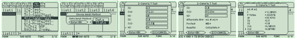
TI-89: Go to the [Apps] Stat/List Editor, then press [2^nd] then F5 [Ints], then select 4: 2-SampTInt. Enter the sample means, sample standard deviations, sample sizes (or list names (list3 & list4), and Freq1:1 & Freq2:1), confidence level. Highlight the No option under Pooled. Press the [ENTER] key to calculate. The calculator returns the confidence interval. If you have the raw data, select Data and enter the list names.

Summary

Use the z-test only if the population variances (or standard deviations) are given in the problem. Most of the time we do not know these values and will use the t-test. A t-test is used for many applications. We use the t-test for a hypothesis test to see if there is a change in the mean between the groups for dependent samples. We can also use the t-test for a hypothesis test to see if there is a change in the mean for independent samples. Be careful which t-test you use, paying attention to the assumption that the variances are equal or not.

9.3.2.b Equal Variance Method t-Test

This method assumes that we know the population’s standard deviations have approximately the same spread. Be careful with this since both populations could be normally distributed and independent, but one population may be way more spread out (larger variance) then the other so you would want to use the unequal variance version. For this text, we will state in the problem whether or not the population’s variances (or standard deviations) are equal. Also, be careful when distinguishing between when to use the z-test versus t-test, just because we assume the population variances or standard deviations are equal does not mean we know their numeric values. We also need to assume the populations are normally distributed if either sample size is below 30.

If we assume the variances are equal \(\left(\sigma_{1}^{2}=\sigma_{2}^{2}\right)\), the formula for the t test statistic is

\(t=\frac{\left(\bar{x}_{1}-\bar{x}_{2}\right)-\left(\mu_{1}-\mu_{2}\right)}{\sqrt{\left(\frac{\left(n_{1}-1\right) s_{1}^{2}+\left(n_{2}-1\right) s_{2}^{2}}{\left(n_{1}+n_{2}-2\right)}\right)\left(\frac{1}{n_{1}}+\frac{1}{n_{2}}\right)}}\)

Use the t-distribution with pooled degrees of freedom df = n₁ – n₂ – 2.

The value \(s^{2}=\frac{\left(n_{1}-1\right) s_{1}^{2}+\left(n_{2}-1\right) s_{2}^{2}}{\left(n_{1}+n_{2}-2\right)}\) under the square root is called the pooled variance and is a weighted mean of the two sample variances, weighted on the corresponding sample sizes.

In some textbooks, they may find the pooled variance first, then place into the formula as \(t=\frac{\left(\bar{x}_{1}-\bar{x}_{2}\right)-\left(\mu_{1}-\mu_{2}\right)}{\sqrt{\left(\frac{s^{2}}{n_{1}}+\frac{s^{2}}{n_{2}}\right)}}\).

Note: The df formula matches what your calculator gives you when you select Yes under the Pooled option.

The traditional method (or critical value method), the p-value method, and the confidence interval method are performed with steps that are identical to those when performing hypothesis tests for one population.

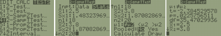
TI-84: Press the [STAT] key, arrow over to the [TESTS] menu, arrow down to the option [4:2-SampTTest] and press the [ENTER] key. Arrow over to the [Stats] menu and press the [Enter] key. Enter the means, standard deviations, sample sizes, confidence level. Then arrow over to the not equal, <, > sign that is the same in the problem’s alternative hypothesis statement, then press the [ENTER] key. Highlight the Yes option under Pooled for unequal variances. Arrow down to [Calculate] and press the [ENTER] key. The calculator returns the test statistic and the p-value. If you have raw data, press the [STAT] key and then the [EDIT] function, enter the data into list one and list two. Press the [STAT] key, arrow over to the [TESTS] menu, arrow down to the option [4:2-SampTTest] and press the [ENTER] key. Arrow over to the [Data] menu and press the [ENTER] key. The defaults are List1: L₁, List2: L₂, Freq1:1, Freq2:1. If these are set different arrow down and use [2^nd] [1] to get L1 and [2^nd] [2] to get L₂.

TI-89: Go to the [Apps] Stat/List Editor, then press [2^nd] then F6 [Tests], then select 4: 2-SampT-Test. Enter the sample means, sample standard deviations, and sample sizes (or list names (list3 & list4), and Freq1:1 & Freq2:1). Then arrow over to the not equal, and select the sign that is the same in the problem’s alternative hypothesis statement. Highlight the Yes option under Pooled. Press the [ENTER] key to calculate. The calculator returns the ttest statistic and the p-value.

Two-Sample t-Interval Assuming Equal Variances

For independent samples, we take the mean of each sample, then take the difference in the means. If the means are equal, then the difference of the two means would be equal to zero. We can then compare the null hypothesis, that there is no difference in the means μ₁ – μ₂ = 0, with the confidence interval limits to decide whether to reject the null hypothesis. If zero is contained within the confidence interval, then we fail to reject H₀. If zero is not contained within the confidence interval, then we reject H₀.

A (1 – \(\alpha\))*100% confidence interval for the difference between two population means µ₁ – µ₂ for independent samples with unequal variances:

\(\left(\bar{x}_{1}-\bar{x}_{2}\right) \pm t_{\alpha / 2} \sqrt{\left(\left(\frac{\left(n_{1}-1\right) s_{1}^{2}+\left(n_{2}-1\right) s_{2}^{2}}{\left(n_{1}+n_{2}-2\right)}\right)\left(\frac{1}{n_{1}}+\frac{1}{n_{2}}\right)\right)}\)

The requirements and degrees of freedom are identical to the above hypothesis test.

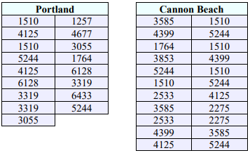
A manager believes that the average sales in coffee at their Portland store is more than the average sales at their Cannon Beach store. They take a random sample of weekly sales from the two stores over the last year. Assume that the sales are normally distributed with equal variances. Use the p-value method with α = 0.05 to test the manager’s claim.

Solution

Assumptions: The sample sizes are both less than 30, but the problem states that the populations are normally distributed. We are testing two means. We do not have population standard deviations or variances given in the problem so this will be a t-test not a z-test. The sales at each store are independent and the problem states that we are assuming, \(\sigma_{1}^{2}=\sigma_{2}^{2}\).

Set up the hypotheses, where group 1 is Portland, and group 2 is Cannon Beach.

We want to test if the Portland mean > Cannon Beach mean, so carry this sign down to the alternative hypothesis to get a right-tailed test:

H₀: µ₁ = µ₂

H₁: µ₁ > µ₂.

Use technology to compute the sample means, standard deviations and sample sizes to get the following test statistic.

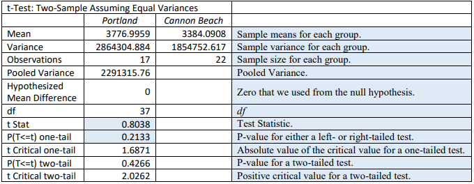
\(t=\frac{\left(\bar{x}_{1}-\bar{x}_{2}\right)-\left(\mu_{1}-\mu_{2}\right)_{0}}{\sqrt{\left(\frac{\left(n_{1}-1\right) s_{1}^{2}+\left(n_{2}-1\right) s_{2}^{2}}{\left(n_{1}+n_{2}-2\right)}\right)\left(\frac{1}{n_{1}}+\frac{1}{n_{2}}\right)}}=\frac{(3776.9959-3384.0908)-0}{\sqrt{\left(\left(\frac{(16 * 2864304.884+21 * 1854752.617)}{(17+22-2)}\right)\left(\frac{1}{17}+\frac{1}{22}\right)\right)}}=0.8038\)

The df = n₁ + n₂ – 1. To find the p-value using the TI calculator DIST menu with tcdf(0.8038,1E99,37) or in Excel using =1-T.DIST(0.8038,37,TRUE) = 0.2133.

The p-value = 0.2133 is larger than \(\alpha\) = 0.05, therefore we do not reject H₀.

There is not enough evidence to conclude that there is a significant difference in the average sales for Portland and Cannon Beach.

Excel: Follow the same steps with the Data Analysis tool, except choose the t-Test: Two-Sample Assuming Equal Variances.

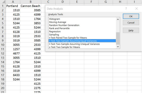
Enter the necessary information as we did in previous sections (see output below) and select OK.

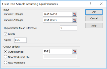
You can only use this Excel shortcut if you have raw data given in the question.

You get the following output:

When reading the Excel output for a z or t-test, be careful with your signs.

• For a left-tailed t-test the critical value will be negative.
• For a right-tailed t-test the critical value will be positive.
• For a two-tailed t-test then your critical values would be ±critical value.

TI-84: Press the [STAT] key, arrow over to the [TESTS] menu, arrow down to the option [0:2-SampTInt] and press the [ENTER] key. Arrow over to the [Stats] menu and press the [Enter] key. Enter the means, sample standard deviations, sample sizes, confidence level. Highlight the Yes option under Pooled for unequal variances. Arrow down to [Calculate] and press the [ENTER] key. The calculator returns the confidence interval.

Or (if you have raw data in list one and list two) press the [STAT] key and then the [EDIT] function, type the data into list one for sample one and list two for sample two. Press the [STAT] key, arrow over to the [TESTS] menu, arrow down to the option [0:2-SampTInt] and press the [ENTER] key. Arrow over to the [Data] menu and press the [ENTER] key. The defaults are List1: L₁ , List2: L₂ , Freq1:1, Freq2:1. If these are set different, arrow down and use [2^nd] [1] to get L₁ and [2^nd] [2] to get L₂ . Then type in the confidence level. Highlight the Yes option under Pooled for unequal variances. Arrow down to [Calculate] and press the [ENTER] key. The calculator returns the confidence interval.

TI-89: Go to the [Apps] Stat/List Editor, then press [2nd] then F5 [Ints], then select 4: 2-SampTInt. Enter the sample means, sample standard deviations, sample sizes (or list names (list3 & list4) and Freq1:1 & Freq2:1), confidence level. Highlight the Yes option under Pooled. Press the [ENTER] key to calculate. The calculator returns the confidence interval. If you have the raw data, select Data and enter the list names as in the following example to the right.