8.4: Hypothesis Test for One Proportion

Last updated
Save as PDF

Page ID: 24058

\( \newcommand{\vecs}[1]{\overset { \scriptstyle \rightharpoonup} {\mathbf{#1}} } \) \( \newcommand{\vecd}[1]{\overset{-\!-\!\rightharpoonup}{\vphantom{a}\smash {#1}}} \)\(\newcommand{\id}{\mathrm{id}}\) \( \newcommand{\Span}{\mathrm{span}}\) \( \newcommand{\kernel}{\mathrm{null}\,}\) \( \newcommand{\range}{\mathrm{range}\,}\) \( \newcommand{\RealPart}{\mathrm{Re}}\) \( \newcommand{\ImaginaryPart}{\mathrm{Im}}\) \( \newcommand{\Argument}{\mathrm{Arg}}\) \( \newcommand{\norm}[1]{\| #1 \|}\) \( \newcommand{\inner}[2]{\langle #1, #2 \rangle}\) \( \newcommand{\Span}{\mathrm{span}}\) \(\newcommand{\id}{\mathrm{id}}\) \( \newcommand{\Span}{\mathrm{span}}\) \( \newcommand{\kernel}{\mathrm{null}\,}\) \( \newcommand{\range}{\mathrm{range}\,}\) \( \newcommand{\RealPart}{\mathrm{Re}}\) \( \newcommand{\ImaginaryPart}{\mathrm{Im}}\) \( \newcommand{\Argument}{\mathrm{Arg}}\) \( \newcommand{\norm}[1]{\| #1 \|}\) \( \newcommand{\inner}[2]{\langle #1, #2 \rangle}\) \( \newcommand{\Span}{\mathrm{span}}\)\(\newcommand{\AA}{\unicode[.8,0]{x212B}}\)

When you read a question, it is essential that you correctly identify the parameter of interest. The parameter determines which model to use. Make sure that you can recognize and distinguish between a question regarding a population mean and a question regarding a population proportion.

The z-test is a statistical test for a population proportion. It can be used when np ≥ 10 and nq ≥ 10.

Definition: z-Test

The formula for the test statistic is:

\[Z=\dfrac{\hat{p}-p_{0}}{\sqrt{\left(\dfrac{p_{0} q_{0}}{n}\right)}}.\]

where

\(n\) is the sample size

\(\hat{p}=\dfrac{x}{n}\) is the sample proportion (sometimes already given as a %) and

\(p_0\) is the hypothesized population proportion,

\[q_0 = 1 – p_0. \nonumber\]

Use the phrases in Figure 8-24 to help with setting up the hypotheses.

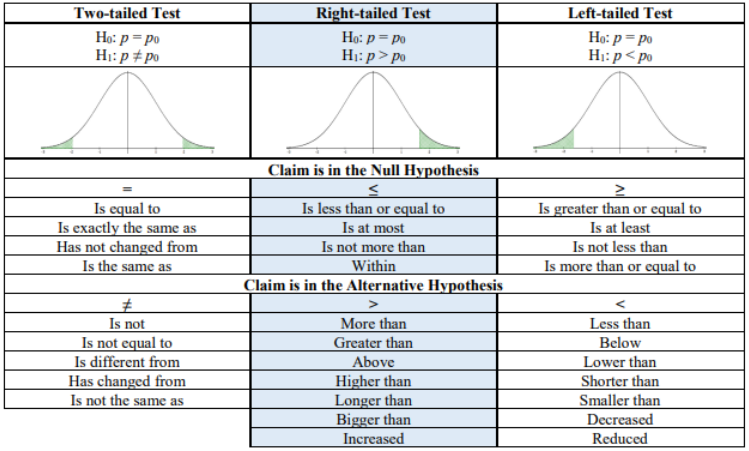
Figure 8-24

Note we will not be using the t-distribution with proportions. We will use a standard normal z distribution for testing a proportion since this test uses the normal approximation to the binomial distribution (never use the t-distribution).

If you are doing a left-tailed z-test the critical value will be negative. If you are performing a right-tailed z-test the critical value will be positive. If you were performing a two-tailed z-test then your critical values would be ±critical value. The p-value will always be a positive number between 0 and 1. The most important step in any method you use is setting up your null and alternative hypotheses. The critical values and p-value can be found using a standard normal distribution the same way that we did for the one sample z-test.

It has been found that 85.6% of all enrolled college and university students in the United States are undergraduates. A random sample of 500 enrolled college students in a particular state revealed that 420 of them were undergraduates. Is there sufficient evidence to conclude that the proportion differs from the national percentage? Use \(\alpha\) = 0.05. Show that all three methods of hypothesis testing yield the same results.

Solution

At this point you should be more comfortable with the steps of a hypothesis test and not have to number each step, but know what each step means.

Critical Value Method

Step 1: State the hypotheses: The key words in this example, “proportion” and “differs,” give the hypotheses:

H₀: p = 0.856

H₁: p ≠ 0.856 (claim)

Step 2: Compute the test statistic. Before finding the test statistic, find the sample proportion \(\hat{p}=\dfrac{420}{500}=0.84\) and q₀ = 1 – 0.856 = 0.144.

Next, compute the test statistic:

\[z=\dfrac{\hat{p}-p_{0}}{\sqrt{\left(\dfrac{p_{0} q_{0}}{n}\right)}}=\dfrac{0.84-0.856}{\sqrt{\left(\dfrac{0.856 \cdot 0.144}{500}\right)}}=-1.019.\]

Step 3: Draw and label the curve with the critical values. See Figure 8-25.

Use \(\alpha\) = 0.05 and technology to compute the critical values \(z_{\alpha / 2}\) and \(z_{1-\alpha / 2}\).

Excel: \(z_{\alpha / 2}\) =NORM.S.INV(0.025) = –1.96 and \(z_{1-\alpha / 2}\) =NORM.S.INV(0.975) = 1.96.

TI-Calculator: \(z_{\alpha / 2}\) = invNorm(0.025,0,1) = –1.96 and \(z_{1-\alpha / 2}\) = invNorm(0.975,0,1) = 1.96.

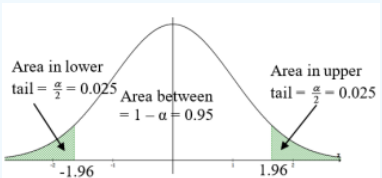
Figure 8-25

Step 4: State the decision. Since the test statistic is not in the shaded rejection area, do not reject H₀.

Step 5: State the summary. At the 5% level of significance, there is not enough evidence to conclude that the proportion of undergraduates in college for this state differs from the national average of 85.6%.

P-value Method

The hypotheses and test statistic stay the same.

H₀: p = 0.856

H₁: p ≠ 0.856 (claim)

\(Z=\dfrac{\hat{p}-p_{0}}{\sqrt{\left(\dfrac{p_{0} q_{0}}{n}\right)}}=\dfrac{0.84-0.856}{\sqrt{\left(\dfrac{0.856 \cdot 0.144}{500}\right)}}=-1.019\)

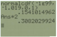
To find the p-value we need to find the P(Z > |1.019|) the area to the left of z = –1.019 and to the right of z = 1.019. First, find the area below (since the test statistic is negative) z = –1.019 using the normalcdf we get 0.1541. Then, double this area to get the p-value = 0.3082.

Since the p-value > \(\alpha\) the decision is to not reject H₀.

Summary: There is not enough evidence to conclude that the proportion of undergraduates in college for this state differs from the national average of 85.6%.

There is a shortcut for this test on the TI Calculators, which will quickly find the test statistic and p-value.

The rejection rule for the two methods are:

P-value method: reject H₀ when the p-value ≤ \(\alpha\).
Critical value method: reject H₀ when the test statistic is in the critical region.

TI-84: Press the [STAT] key, arrow over to the [TESTS] menu, arrow down to the option [5:1-PropZTest] and press the [ENTER] key. Type in the hypothesized proportion (p₀), x, sample size, arrow over to the \(\neq\), <, > sign that is the same in the problem’s alternative hypothesis statement then press the [ENTER] key, arrow down to [Calculate] and press the [ENTER] key.

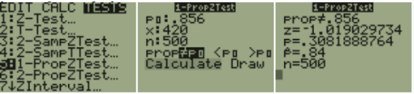
The calculator returns the z-test statistic and the p-value. Note: sometimes you are not given the x value but a percentage instead. To find the x to use in the calculator, multiply \(\hat{p}\) by the sample size and round off to the nearest integer. The calculator will give you an error message if you put in a decimal for x or n. For example, if \(\hat{p}\)= 0.22 and n = 124 then 0.22*124 = 27.28, so use x = 27.

TI-89: Go to the [Apps] Stat/List Editor, then press [2nd] then F6 [Tests], then select 5: 1-PropZ-Test. Type in the hypothesized proportion (p0), x, sample size, arrow over to the \(\neq\), <, > sign that is the same in the problem’s alternative hypothesis statement then press the [ENTER] key to calculate. The calculator returns the z-test statistic and the pvalue. Note: sometimes you are not given the x value but a percentage instead. To find the x value to use in the calculator, multiply \(\hat{p}\) by the sample size and round off to the nearest integer. The calculator will give you an error message if you put in a decimal for x or n. For example, if \(\hat{p}\) = 0.22 and n = 124 then 0.22*124 = 27.28, so use x = 27.