
5.6: Poisson Distribution
- Page ID
- 26589

\( \newcommand{\vecs}[1]{\overset { \scriptstyle \rightharpoonup} {\mathbf{#1}} } \)
\( \newcommand{\vecd}[1]{\overset{-\!-\!\rightharpoonup}{\vphantom{a}\smash {#1}}} \)
\( \newcommand{\dsum}{\displaystyle\sum\limits} \)
\( \newcommand{\dint}{\displaystyle\int\limits} \)
\( \newcommand{\dlim}{\displaystyle\lim\limits} \)
\( \newcommand{\id}{\mathrm{id}}\) \( \newcommand{\Span}{\mathrm{span}}\)
( \newcommand{\kernel}{\mathrm{null}\,}\) \( \newcommand{\range}{\mathrm{range}\,}\)
\( \newcommand{\RealPart}{\mathrm{Re}}\) \( \newcommand{\ImaginaryPart}{\mathrm{Im}}\)
\( \newcommand{\Argument}{\mathrm{Arg}}\) \( \newcommand{\norm}[1]{\| #1 \|}\)
\( \newcommand{\inner}[2]{\langle #1, #2 \rangle}\)
\( \newcommand{\Span}{\mathrm{span}}\)
\( \newcommand{\id}{\mathrm{id}}\)
\( \newcommand{\Span}{\mathrm{span}}\)
\( \newcommand{\kernel}{\mathrm{null}\,}\)
\( \newcommand{\range}{\mathrm{range}\,}\)
\( \newcommand{\RealPart}{\mathrm{Re}}\)
\( \newcommand{\ImaginaryPart}{\mathrm{Im}}\)
\( \newcommand{\Argument}{\mathrm{Arg}}\)
\( \newcommand{\norm}[1]{\| #1 \|}\)
\( \newcommand{\inner}[2]{\langle #1, #2 \rangle}\)
\( \newcommand{\Span}{\mathrm{span}}\) \( \newcommand{\AA}{\unicode[.8,0]{x212B}}\)
\( \newcommand{\vectorA}[1]{\vec{#1}} % arrow\)
\( \newcommand{\vectorAt}[1]{\vec{\text{#1}}} % arrow\)
\( \newcommand{\vectorB}[1]{\overset { \scriptstyle \rightharpoonup} {\mathbf{#1}} } \)
\( \newcommand{\vectorC}[1]{\textbf{#1}} \)
\( \newcommand{\vectorD}[1]{\overrightarrow{#1}} \)
\( \newcommand{\vectorDt}[1]{\overrightarrow{\text{#1}}} \)
\( \newcommand{\vectE}[1]{\overset{-\!-\!\rightharpoonup}{\vphantom{a}\smash{\mathbf {#1}}}} \)
\( \newcommand{\vecs}[1]{\overset { \scriptstyle \rightharpoonup} {\mathbf{#1}} } \)
\(\newcommand{\longvect}{\overrightarrow}\)
\( \newcommand{\vecd}[1]{\overset{-\!-\!\rightharpoonup}{\vphantom{a}\smash {#1}}} \)
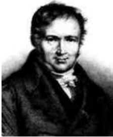
\(\newcommand{\avec}{\mathbf a}\) \(\newcommand{\bvec}{\mathbf b}\) \(\newcommand{\cvec}{\mathbf c}\) \(\newcommand{\dvec}{\mathbf d}\) \(\newcommand{\dtil}{\widetilde{\mathbf d}}\) \(\newcommand{\evec}{\mathbf e}\) \(\newcommand{\fvec}{\mathbf f}\) \(\newcommand{\nvec}{\mathbf n}\) \(\newcommand{\pvec}{\mathbf p}\) \(\newcommand{\qvec}{\mathbf q}\) \(\newcommand{\svec}{\mathbf s}\) \(\newcommand{\tvec}{\mathbf t}\) \(\newcommand{\uvec}{\mathbf u}\) \(\newcommand{\vvec}{\mathbf v}\) \(\newcommand{\wvec}{\mathbf w}\) \(\newcommand{\xvec}{\mathbf x}\) \(\newcommand{\yvec}{\mathbf y}\) \(\newcommand{\zvec}{\mathbf z}\) \(\newcommand{\rvec}{\mathbf r}\) \(\newcommand{\mvec}{\mathbf m}\) \(\newcommand{\zerovec}{\mathbf 0}\) \(\newcommand{\onevec}{\mathbf 1}\) \(\newcommand{\real}{\mathbb R}\) \(\newcommand{\twovec}[2]{\left[\begin{array}{r}#1 \\ #2 \end{array}\right]}\) \(\newcommand{\ctwovec}[2]{\left[\begin{array}{c}#1 \\ #2 \end{array}\right]}\) \(\newcommand{\threevec}[3]{\left[\begin{array}{r}#1 \\ #2 \\ #3 \end{array}\right]}\) \(\newcommand{\cthreevec}[3]{\left[\begin{array}{c}#1 \\ #2 \\ #3 \end{array}\right]}\) \(\newcommand{\fourvec}[4]{\left[\begin{array}{r}#1 \\ #2 \\ #3 \\ #4 \end{array}\right]}\) \(\newcommand{\cfourvec}[4]{\left[\begin{array}{c}#1 \\ #2 \\ #3 \\ #4 \end{array}\right]}\) \(\newcommand{\fivevec}[5]{\left[\begin{array}{r}#1 \\ #2 \\ #3 \\ #4 \\ #5 \\ \end{array}\right]}\) \(\newcommand{\cfivevec}[5]{\left[\begin{array}{c}#1 \\ #2 \\ #3 \\ #4 \\ #5 \\ \end{array}\right]}\) \(\newcommand{\mattwo}[4]{\left[\begin{array}{rr}#1 \amp #2 \\ #3 \amp #4 \\ \end{array}\right]}\) \(\newcommand{\laspan}[1]{\text{Span}\{#1\}}\) \(\newcommand{\bcal}{\cal B}\) \(\newcommand{\ccal}{\cal C}\) \(\newcommand{\scal}{\cal S}\) \(\newcommand{\wcal}{\cal W}\) \(\newcommand{\ecal}{\cal E}\) \(\newcommand{\coords}[2]{\left\{#1\right\}_{#2}}\) \(\newcommand{\gray}[1]{\color{gray}{#1}}\) \(\newcommand{\lgray}[1]{\color{lightgray}{#1}}\) \(\newcommand{\rank}{\operatorname{rank}}\) \(\newcommand{\row}{\text{Row}}\) \(\newcommand{\col}{\text{Col}}\) \(\renewcommand{\row}{\text{Row}}\) \(\newcommand{\nul}{\text{Nul}}\) \(\newcommand{\var}{\text{Var}}\) \(\newcommand{\corr}{\text{corr}}\) \(\newcommand{\len}[1]{\left|#1\right|}\) \(\newcommand{\bbar}{\overline{\bvec}}\) \(\newcommand{\bhat}{\widehat{\bvec}}\) \(\newcommand{\bperp}{\bvec^\perp}\) \(\newcommand{\xhat}{\widehat{\xvec}}\) \(\newcommand{\vhat}{\widehat{\vvec}}\) \(\newcommand{\uhat}{\widehat{\uvec}}\) \(\newcommand{\what}{\widehat{\wvec}}\) \(\newcommand{\Sighat}{\widehat{\Sigma}}\) \(\newcommand{\lt}{<}\) \(\newcommand{\gt}{>}\) \(\newcommand{\amp}{&}\) \(\definecolor{fillinmathshade}{gray}{0.9}\)The Poisson distribution was named after the French mathematician Siméon Poisson (pronounced pwɑːsɒn, means fish in French).
The Poisson discrete probability distribution finds the probability of an event over some unit of time or space. A Poisson probability distribution may be used when a random experiment meets all of the following requirements.
- Events occur independently.
- The discrete random variable X is the number of occurrences over an interval of time, volume, space, area, etc.
- The mean number of successes μ over time, volume, space, area, etc. is given. (Note some textbooks and calculators use lambda = λ instead of mu = μ for the mean).
The formula for the Poisson distribution is P(X = x) = \(\frac{e^{-\mu} \mu^{x}}{x !}\), where e is a mathematical constant approximately equal to 2.71828, x = 0, 1, 2, … is the number successes that you are trying to find the probability for, μ is the mean number of a success over one interval of time, space, volume, etc.
The value of x has no stopping point since there is no set sample size like the binomial distribution. Note that e is not a variable, it is a constant number. Use the ex button on your calculator.
Mean, Variance & Standard Deviation of a Poisson Distribution
For a Poisson distribution, μ, the expected number of successes, and the variance σ2 are equal to one another.
\(\mu=\sigma^{2} \quad \sigma=\sqrt{\sigma^{2}}\)
Sometimes the question will ask for a probability over a different unit of time, space or area than originally given in the problem. Always change the mean to fit the new units in the question.
This formula will help in correctly rescaling the mean to fit the questions new units: New μ = old μ(\(\frac {\text {new units}}{\text {old units}}\)). The “old” would be the original stated mean and units and the “new” is the units from the question.
TI-84: Press [2nd] [DISTR]. This will get you a menu of probability distributions. Press [ALPHA] B or arrow down to B:poissonpdf( and press [ENTER]. This puts poissonpdf( on the home screen. Enter the values for μ and x with a comma between each. Press [ENTER]. This is the probability density function and will return you the probability of exactly x successes. Press [ALPHA] C or arrow down to C:poissoncdf( and press [ENTER]. This puts poissoncdf( on the home screen. Enter the values for μ and x with a comma between each. Press [ENTER]. This is the cumulative distribution function and will return you the probability of at most x successes.
TI-89: Go to the [Apps] Stat/List Editor, then select F5 [DISTR]. This will get you a menu of probability distributions. Arrow down to Poisson Pdf and press [ENTER]. Enter the values for μ and x into each cell. Press [ENTER]. This is the probability density function and will return you the probability of exactly x successes. Arrow down to Poisson Cdf and press [ENTER]. Enter the values for μ and the lower and upper values of x into each cell. Press [ENTER]. This is the cumulative distribution function and will return you the probability between the lower and upper x-values, inclusive.
Excel: Use the formula =POISSON.DIST(x,mean,false) for P(X = x). Use the formula =POISSON.DIST(x,mean,true) for P(X ≤ x).
There are about 8 million individuals in New York City. Using historical records, the average number of individuals hospitalized for acute myocardial infarction (AMI), i.e. a heart attack, each day is 4.4 individuals. What is the probability that exactly 6 people are hospitalized for AMI in NY City tomorrow?
Solution
First, note that the probability question is over the same units of time, one day, which the average is given. It is important that these units always match. The random variable X = the number of individuals hospitalized each day in NY City for an AMI.
We are trying to find P(X = 6) and the mean μ = 4.4 people.
Using the formula P(X = 6) = \(\frac{e^{-4.4} 4.4^{6}}{6 !}\) = 0.1237.
TI-84: poissonpdf(4.4,6) = 0.1237.
Excel =POISSON.DIST(6,4.4,FALSE) = 0.1237.
A bank drive-through has an average of 10 customers every hour. Find the following probabilities.
a) Compute the probability that no customers arrive in an hour.
b) Compute the probability of exactly 2 customers use the drive-through in an hour.
c) Compute the probability that exactly 2 customers use the drive-through in a 30-minute period.
d) Compute the probability that fewer than 2 customers use the drive-through in a half hour.
Solution
a) In this case, X is the number of customers that use the drive-through. We are trying to find the probability that x = 0. The average is given in the problem as μ = 10. This gives P(X = 0) = \(\frac{e^{-10} 10^{0}}{0 !}\) = 4.53999E-5 = 0.0000454.
TI-84: poissonpdf(10,0) = 0.0000454.
Excel: =POISSON.DIST(0,10,FALSE) = 0.0000454.
b) P(X = 2) = \(\frac{e^{-10} 10^{2}}{2 !}\) = 0.0023.
TI-84: P(X = 2) = poissonpdf(10,2) = 0.0023.
Excel: =POISSON.DIST(2,10,FALSE) = 0.0023.
c) The unit of time has changed from 1 hour to 30 minutes, so we need to rescale the mean to fit the new unit of time. Use the following formula to convert your units, New μ = old μ(\(\frac {\text {new units}}{\text {old units}}\)) = 10(\(\frac {\text {30 minutes}}{\text {60 minutes}}\)) = 5.
P(X = 2) = \(\frac{e^{-5} 5^{2}}{2 !}\) = 0.0842.
TI-84: P(X = 2) = poissonpdf(5,2) = 0.0842.
Excel: P(X = 2) =POISSON.DIST(2,5,FALSE) = 0.0842.
Note; always rescale the mean to fit the units of the question, not the other way around.
d) The time-period is half an hour = 30 minutes. The mean from part c would be μ = 5. To find “less than” 2 we would have zero or one customer.
P(X < 2) = P(X = 0) + P(X =1) = \(\frac{e^{-5} 5^{0}}{0 !}\) + \(\frac{e^{-5} 5^{1}}{1 !}\) = = 0.0067 + 0.0337 = 0.0404.
TI-84: P(X = 2) = poissoncdf(5,1) = 0.0404.
Excel: =POISSON.DIST(1,5,TRUE) = 0.0404.
So far, most of the examples for the Poisson distribution were for exactly x successes. If we want to find the probability of accumulation of x values then we would use the cumulative distribution function (cdf) instead of the pdf. As you read through a problem look for some of the following key phrases in Figure 5-9. Once you find the phrase then match up to what sign you would use and then use the table to walk you through the computer or calculator formula.
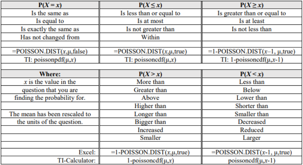
Figure 5-9
A bank drive-through has an average of 10 customers every hour. Find the following probabilities.
a) Compute the probability of at least four customers arriving in an hour.
b) Compute the probability of at most four customers arriving in an hour.
c) Compute the probability of fewer than four customers arriving in an hour.
d) Compute the probability of more than four customers arriving in an hour.
e) Compute the probability that fewer than 2 customers arrive in a 15-minute period.
Solution
a) Because we do not have a set sample size to stop at like the binomial distribution, you would have to find the probability of 4 or more until your answers are small enough that they are not changing your answer out to at least four decimal places 0.0000. This may take a lot of work; instead, we will use the complement rule. The complement to “at least 4,” is “3 or less.” Find P(X ≥ 4) = 1 – P(X ≤ 3) = 1 – P(X = 0) + P(X = 1) + P(X = 2) + P(X = 3) = \(1-\left(\frac{e^{-10} 10^{0}}{0 !}+\frac{e^{-10} 10^{1}}{1 !}+\frac{e^{-10} 10^{2}}{2 !}+\frac{e^{-10} 10^{3}}{3 !}\right)\) = 1 – 0.000045 + 0.000454 + 0.00227 + 0.007567 = 1 – 0.0103 = 0.9897. Note that the value of x went from 4 to 3. The complement of strictly less than 4 starts at x = 3.
TI-84: 1 – poissoncdf(10,3) = 0.9897.
Excel: =1-POISSON.DIST(3,10,TRUE) = 0.9897.
b) P(X ≤ 4) = P(X = 0) + P(X = 1) + P(X = 2) + P(X = 3) + P(X = 4) = \(\frac{e^{-10} 10^{0}}{0 !}+\frac{e^{-10} 10^{1}}{1 !}+\frac{e^{-10} 10^{2}}{2 !}+\frac{e^{-10} 10^{3}}{3 !}+\frac{e^{-10} 10^{4}}{4 !}\) = 0.000045 + 0.000454 + 0.00227 + 0.007567 + 0.018917 = 0.0293.
TI-84: poissoncdf(10,4) = 0.0293.
Excel: =POISSON.DIST(4,10,TRUE) = 0.0293.
c) P(X < 4) = P(X = 0) + P(X = 1) + P(X = 2) + P(X = 3) = \(\frac{e^{-10} 10^{0}}{0 !}+\frac{e^{-10} 10^{1}}{1 !}+\frac{e^{-10} 10^{2}}{2 !}+\frac{e^{-10} 10^{3}}{3 !}\) 0.000045 + 0.000454 + 0.00227 + 0.007567 = 0.0103.
TI-84: poissoncdf(10,3) = 0.0103.
Excel: =POISSON.DIST(3,10,TRUE) = 0.0103.
d) Using part b, P(X > 4) = 1 – P(X ≤ 4) = 1 – 0.0293 = 0.9707.
TI-84: 1 – poissoncdf(10,4) = 0.9707.
Excel: =1-POISSON.DIST(4,10,TRUE) = 0.9707.
e) The unit of time has changed from 1 hour to 15 minutes, so we need to rescale the mean to fit the new unit of time. Use the following formula to convert your units, New μ = old μ(\(\frac {\text {new units}}{\text {old units}}\)) = 10(\(\frac {\text {15 minutes}}{\text {60 minutes}}\)) = 2.5.
P(X < 2) = P(X = 0) + P(X = 1) = \(\frac{e^{-2.5} 2.5^{0}}{0 !}\) + \(\frac{e^{-2.5} 2.5^{1}}{1 !}\) = 0.0821 + 0.2052 = 0.2873.
TI-84: poissoncdf(2.5,1) = 0.2873.
Excel: =POISSON.DIST(1,2.5,TRUE) = 0.2873.
The last ever dolphin message was misinterpreted as a surprisingly sophisticated attempt to do a double--‐ backwards – somersault through a hoop whilst whistling the "Star Sprangled Banner," but in fact the message was this: So long and thanks for all the fish.
(Adams, 2002)