8.2: The Central Limit Theorem for Sample Proportions
- Page ID
- 20900
\( \newcommand{\vecs}[1]{\overset { \scriptstyle \rightharpoonup} {\mathbf{#1}} } \)
\( \newcommand{\vecd}[1]{\overset{-\!-\!\rightharpoonup}{\vphantom{a}\smash {#1}}} \)
\( \newcommand{\id}{\mathrm{id}}\) \( \newcommand{\Span}{\mathrm{span}}\)
( \newcommand{\kernel}{\mathrm{null}\,}\) \( \newcommand{\range}{\mathrm{range}\,}\)
\( \newcommand{\RealPart}{\mathrm{Re}}\) \( \newcommand{\ImaginaryPart}{\mathrm{Im}}\)
\( \newcommand{\Argument}{\mathrm{Arg}}\) \( \newcommand{\norm}[1]{\| #1 \|}\)
\( \newcommand{\inner}[2]{\langle #1, #2 \rangle}\)
\( \newcommand{\Span}{\mathrm{span}}\)
\( \newcommand{\id}{\mathrm{id}}\)
\( \newcommand{\Span}{\mathrm{span}}\)
\( \newcommand{\kernel}{\mathrm{null}\,}\)
\( \newcommand{\range}{\mathrm{range}\,}\)
\( \newcommand{\RealPart}{\mathrm{Re}}\)
\( \newcommand{\ImaginaryPart}{\mathrm{Im}}\)
\( \newcommand{\Argument}{\mathrm{Arg}}\)
\( \newcommand{\norm}[1]{\| #1 \|}\)
\( \newcommand{\inner}[2]{\langle #1, #2 \rangle}\)
\( \newcommand{\Span}{\mathrm{span}}\) \( \newcommand{\AA}{\unicode[.8,0]{x212B}}\)
\( \newcommand{\vectorA}[1]{\vec{#1}} % arrow\)
\( \newcommand{\vectorAt}[1]{\vec{\text{#1}}} % arrow\)
\( \newcommand{\vectorB}[1]{\overset { \scriptstyle \rightharpoonup} {\mathbf{#1}} } \)
\( \newcommand{\vectorC}[1]{\textbf{#1}} \)
\( \newcommand{\vectorD}[1]{\overrightarrow{#1}} \)
\( \newcommand{\vectorDt}[1]{\overrightarrow{\text{#1}}} \)
\( \newcommand{\vectE}[1]{\overset{-\!-\!\rightharpoonup}{\vphantom{a}\smash{\mathbf {#1}}}} \)
\( \newcommand{\vecs}[1]{\overset { \scriptstyle \rightharpoonup} {\mathbf{#1}} } \)
\( \newcommand{\vecd}[1]{\overset{-\!-\!\rightharpoonup}{\vphantom{a}\smash {#1}}} \)
\(\newcommand{\avec}{\mathbf a}\) \(\newcommand{\bvec}{\mathbf b}\) \(\newcommand{\cvec}{\mathbf c}\) \(\newcommand{\dvec}{\mathbf d}\) \(\newcommand{\dtil}{\widetilde{\mathbf d}}\) \(\newcommand{\evec}{\mathbf e}\) \(\newcommand{\fvec}{\mathbf f}\) \(\newcommand{\nvec}{\mathbf n}\) \(\newcommand{\pvec}{\mathbf p}\) \(\newcommand{\qvec}{\mathbf q}\) \(\newcommand{\svec}{\mathbf s}\) \(\newcommand{\tvec}{\mathbf t}\) \(\newcommand{\uvec}{\mathbf u}\) \(\newcommand{\vvec}{\mathbf v}\) \(\newcommand{\wvec}{\mathbf w}\) \(\newcommand{\xvec}{\mathbf x}\) \(\newcommand{\yvec}{\mathbf y}\) \(\newcommand{\zvec}{\mathbf z}\) \(\newcommand{\rvec}{\mathbf r}\) \(\newcommand{\mvec}{\mathbf m}\) \(\newcommand{\zerovec}{\mathbf 0}\) \(\newcommand{\onevec}{\mathbf 1}\) \(\newcommand{\real}{\mathbb R}\) \(\newcommand{\twovec}[2]{\left[\begin{array}{r}#1 \\ #2 \end{array}\right]}\) \(\newcommand{\ctwovec}[2]{\left[\begin{array}{c}#1 \\ #2 \end{array}\right]}\) \(\newcommand{\threevec}[3]{\left[\begin{array}{r}#1 \\ #2 \\ #3 \end{array}\right]}\) \(\newcommand{\cthreevec}[3]{\left[\begin{array}{c}#1 \\ #2 \\ #3 \end{array}\right]}\) \(\newcommand{\fourvec}[4]{\left[\begin{array}{r}#1 \\ #2 \\ #3 \\ #4 \end{array}\right]}\) \(\newcommand{\cfourvec}[4]{\left[\begin{array}{c}#1 \\ #2 \\ #3 \\ #4 \end{array}\right]}\) \(\newcommand{\fivevec}[5]{\left[\begin{array}{r}#1 \\ #2 \\ #3 \\ #4 \\ #5 \\ \end{array}\right]}\) \(\newcommand{\cfivevec}[5]{\left[\begin{array}{c}#1 \\ #2 \\ #3 \\ #4 \\ #5 \\ \end{array}\right]}\) \(\newcommand{\mattwo}[4]{\left[\begin{array}{rr}#1 \amp #2 \\ #3 \amp #4 \\ \end{array}\right]}\) \(\newcommand{\laspan}[1]{\text{Span}\{#1\}}\) \(\newcommand{\bcal}{\cal B}\) \(\newcommand{\ccal}{\cal C}\) \(\newcommand{\scal}{\cal S}\) \(\newcommand{\wcal}{\cal W}\) \(\newcommand{\ecal}{\cal E}\) \(\newcommand{\coords}[2]{\left\{#1\right\}_{#2}}\) \(\newcommand{\gray}[1]{\color{gray}{#1}}\) \(\newcommand{\lgray}[1]{\color{lightgray}{#1}}\) \(\newcommand{\rank}{\operatorname{rank}}\) \(\newcommand{\row}{\text{Row}}\) \(\newcommand{\col}{\text{Col}}\) \(\renewcommand{\row}{\text{Row}}\) \(\newcommand{\nul}{\text{Nul}}\) \(\newcommand{\var}{\text{Var}}\) \(\newcommand{\corr}{\text{corr}}\) \(\newcommand{\len}[1]{\left|#1\right|}\) \(\newcommand{\bbar}{\overline{\bvec}}\) \(\newcommand{\bhat}{\widehat{\bvec}}\) \(\newcommand{\bperp}{\bvec^\perp}\) \(\newcommand{\xhat}{\widehat{\xvec}}\) \(\newcommand{\vhat}{\widehat{\vvec}}\) \(\newcommand{\uhat}{\widehat{\uvec}}\) \(\newcommand{\what}{\widehat{\wvec}}\) \(\newcommand{\Sighat}{\widehat{\Sigma}}\) \(\newcommand{\lt}{<}\) \(\newcommand{\gt}{>}\) \(\newcommand{\amp}{&}\) \(\definecolor{fillinmathshade}{gray}{0.9}\)The Central Limit Theorem will also work for sample proportions if certain conditions are met.
The Binomial Distribution
In Chapter 6, we explored the Binomial Random Variable, in which \(X\) measures the number of successes in a fixed number of independent trials. The Binomial distribution had two parameters: the sample size \(n\), and the probability of success on a single trial \(p\).
Example: Free throw shooting
Recall the example of Draymond Green, an NBA basketball player for the Golden State Warriors who is a 70% free throw shooter.
The random variable \(X\) = the number of successes when Draymond Green takes \(n\) free throw follows a Bernoulli Distribution with \(p =0.7\) (success) and \(q = 0.3\) (failure). Let's graph the probability distribution function for \(n\)=1, 5, 25 and 100:
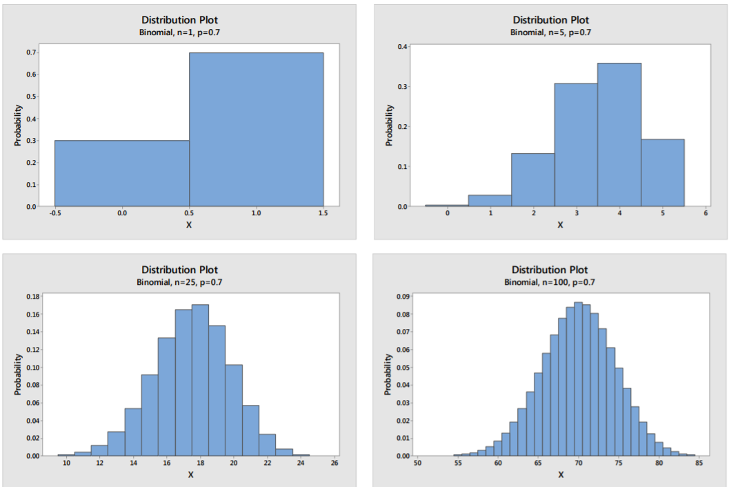
Notice that as the sample size gets larger, the shape of the random variable becomes Normal.
A good rule to use is that if \(np>10\) and \(n(1‐p) > 10\), the shape of the Binomial Distribution is approximately Normal.
The Sample Proportion random variable
Instead of looking at the number of successes in a fixed number, consider the proportion of successes in these trials. We will use the symbol \(\hat{p}\) (read as p‐hat) to represent the proportion of successes in \(n\) trials. If \(X\) is the number of successes in \(n\) trials, \(\hat{p}=\dfrac{X}{n}\) is the sample proportion of successes in \(n\) trials.
Here is a comparison of these two random variables:
Random Variable | \(X\) | \(\hat{p}\) |
---|---|---|
Expected value | \(\mu=n p\) | \(\mu_{\hat{p}}=p\) |
Variance | \(\sigma^{2}=n p(1-p)\) | \(\sigma_{\hat{p}}^{2}=\dfrac{p(1-p)}{n}\) |
Standard Deviation | \(\sigma=\sqrt{n p(1-p)}\) | \(\sigma_{\hat{p}}=\sqrt{\dfrac{p(1-p)}{n}}\) |
Example: Free throw shooting
Draymond Green, a 70% free‐throw shooter, takes 4 free throws.
\(X\) = The number of successes in 4 free throws.
\(\hat{p}=\dfrac{X}{n}\) = The proportion of successes in 4 free throws.
Determine the probability distribution function, the expected value and the standard deviation for the random variable \(\hat{p}\).
Solution
\(x\) | \(\hat{p}\) | \(P(\hat{p})\) |
---|---|---|
0 | 0.00 | 0.0081 |
1 | 0.25 | 0.0756 |
2 | 0.50 | 0.2646 |
3 | 0.75 | 0.3087 |
4 | 1.00 | 0.2401 |
\(\mu_{\hat{p}}=p=0.7\)
\(\sigma_{\hat{p}}=\sqrt{\dfrac{p(1-p)}{n}}=\sqrt{\dfrac{0.7(1-0.7)}{4}}=0.2291\)
The Central Limit Theorem for Sample Proportions
If \(X\) is a Random Variable from a Binomial Distribution with parameters \(n\) and \(p\), and \(np > 10\) and \(n(1‐p) > 10\)
Then the following is true for the Sample Proportion \(\hat{p}=\dfrac{X}{n}\)
- \(\mu_{\hat{p}}=p\)
- \(\sigma_{\hat{p}}=\sqrt{\dfrac{p(1-p)}{n}}\)
- The Distribution of \(\hat{p}\) is approximately Normal.
Combining all of the above into a single formula: \(Z=\dfrac{\hat{p}-p}{\sqrt{\frac{p(1-p)}{n}}}\) where \(Z\) represents the Standard Normal Distribution.
Example: California Community College Fee Waivers
The graph below shows enrollment at California Community Colleges and the percentage of students who are receiving Board of Governors Fee Waivers (BOGFW) to help financially.70
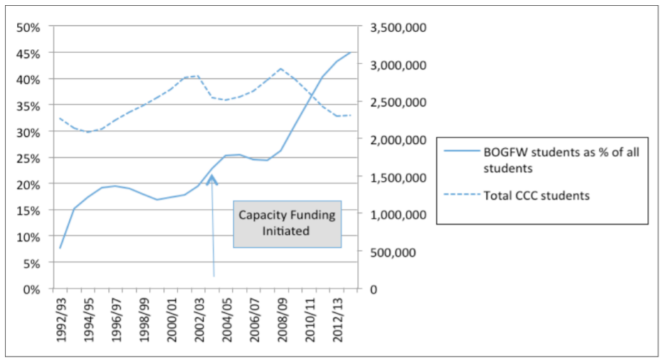
This graph shows that 45% of all community college students in California receive fee waivers. Suppose you randomly sample 1000 community college students to determine the proportion of students with fee waivers in the sample.
\(p\) = 0.45 (the proportion of all community college students with fee waivers)
\(n\) = 1000 ( the sample size)
\(np = (1000)(0.45) = 450 n(1‐p) = (1000)(1‐0.45) = 550\).
Since both these values are over 10, the conditions for normality are met.
\(\hat{p}\) = the proportion of sampled community college students with fee waivers, a random variable
\(\mu_{\hat{p}}=0.45\)
\(\sigma_{\hat{p}}=\sqrt{\dfrac{0.45(1-.045)}{1000}}=0.0157\)
483 of the sampled students are receiving fee waivers.
Determine \(\hat{p}\). Is the result unusual?
Solution
\(\hat{p}=\frac{483}{1000}=0.483\)
\(Z=\frac{0.483-0.45}{0.0157}=2.10\)
\(P(Z>2.10)=0.0179\)
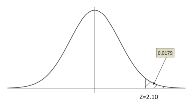
The sample proportion of 0.483 is unusually high, since the \(Z\) value is more than 2. The probability of getting a sample proportion of 0.483 or larger is only 0.0179.