8.1: The Central Limit Theorem for Sample Means

First, think of a random variable \(X\) from a population that is defined by some probability distribution or density function. This random variable could be continuous or discrete data. Sampling is repeatedly obtaining values of this random variable.

We will define a Random Sample \(X_{1}, X_{2}, \ldots, X_{n}\) in which each of the random variables \(X_{i}\) has the same probability distribution and are mutually independent of each other. The sample mean is a function of these random variables (add them up and divide by the sample size), so \(\overline{X}\) is a random variable. So what is the Probability Distribution Function (pdf) of \(\overline{X}\)?

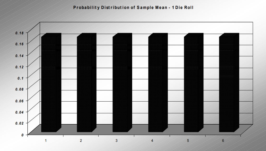
To answer this question, conduct the following experiment. We will roll samples of \(n\) dice, determine the mean roll, and create a pdf for different values of \(n\). For the case \(n=1\), the distribution of the sample mean is the same as the distribution of the random variable. Since each die has the same chance of being chosen, the distribution is rectangular shaped centered at 3.5:

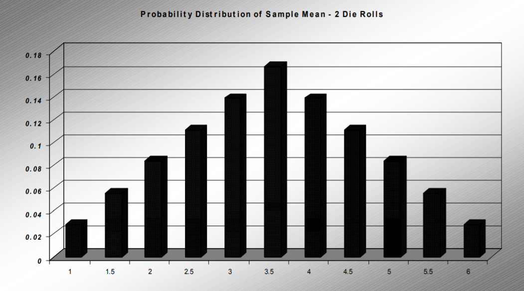
For the case \(n=2\), the distribution of the sample mean starts to take on a triangular shape since some values are more likely to be rolled than others. For example, there are six ways to roll a total of 7 and get a sample mean of 3.5, but only one way to roll a total of 2 and get a sample mean of 1. Notice the pdf is still centered at 3.5.

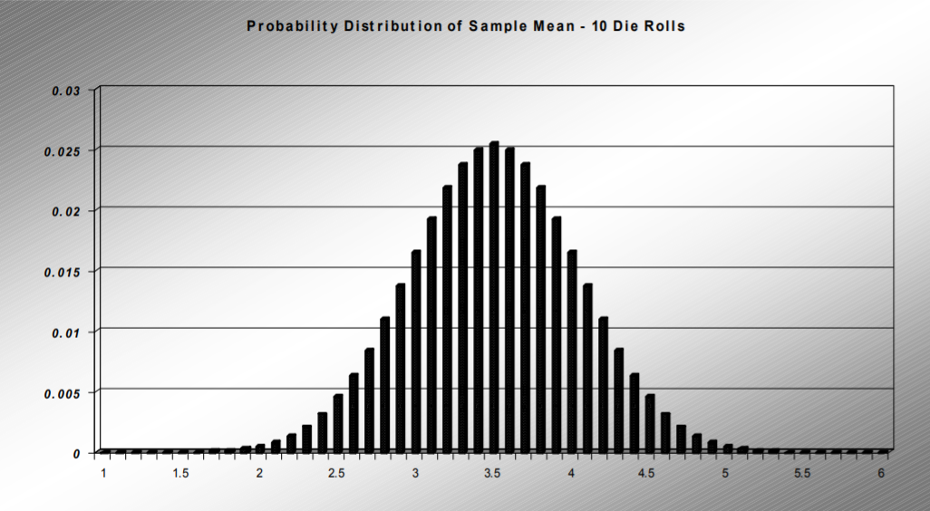
For the case \(n=10\), the pdf of the sample mean   now takes on a familiar bell shape that looks like a Normal Distribution. The center is still at 3.5 and the values are now more tightly clustered around the mean, implying that the standard deviation has decreased. 

Finally, for the case \(n=30\), the pdf continues to look like the Normal Distribution centered around the same mean of 3.5, but more tightly clustered than the prior example:

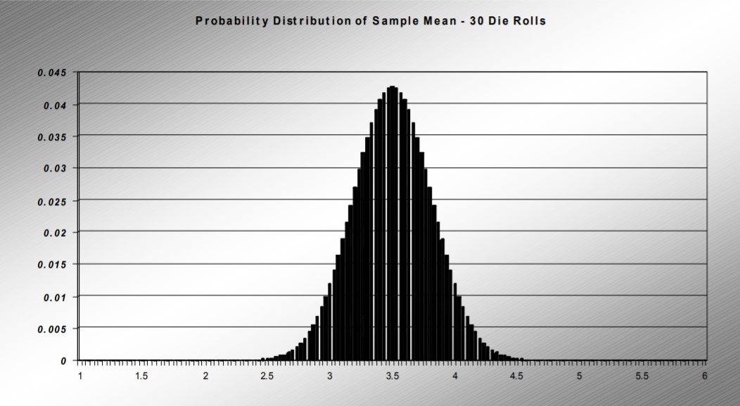
This die‐rolling example demonstrates the Central Limit Theorem’s three important observations about the PDF of \(\overline{X}\) compared to the pdf of the original random variable.

1. The mean stays the same.
2. The standard deviation gets smaller.
3. As the sample size increase, the pdf of \(\overline{X}\) is approximately a Normal Distribution.

Central Limit Theorem for the Sample Mean

If \(X_{1}, X_{2}, \ldots, X_{n}\) is a random sample from a population that has a mean \(\mu\) and a standard deviation \(\sigma\), and \(n\) is sufficiently large (\(n \geq 30\)) then:

1. \(\mu_{\bar{X}}=\mu\)
2. \(\sigma_{\bar{X}}=\dfrac{\sigma}{\sqrt{n}}\)
3. The Distribution of \(\overline{X}\) is approximately Normal.

Combining all of the above into a single formula: \(Z=\dfrac{\overline{X}-\mu}{\sigma / \sqrt{n}}\), where \(Z\) represents the Standard Normal Distribution.

This powerful result allows us to use the sample mean \(\overline{X}\) as an estimator of the population mean \(\mu\). In fact, most inferential statistics practiced today would not be possible without the Central Limit Theorem.

Example: Mean height of men

The mean height of American men (ages 20‐29) is \(\mu = 69.2\) inches. If a random sample of 60 men in this age group is selected, what is the probability the mean height for the sample is greater than 70 inches? Assume \(\sigma=2.9^{\prime \prime}\)

Solution

Due to the Central Limit Theorem, we know the distribution of the Sample will have approximately a Normal Distribution:

\[P(\overline{X}>70)=P\left(Z>\dfrac{(70-69.2)}{2.9 / \sqrt{60}}\right)=P(Z>2.14)=0.0162 \nonumber \]

Compare this to the much larger probability that one male chosen will be over 70 inches tall:

\[P(X>70)=P\left(Z>\dfrac{(70-69.2)}{2.9}\right)=P(Z>0.28)=0.3897 \nonumber \]

This example demonstrates how the sample mean will cluster towards the population mean as the sample size increases.

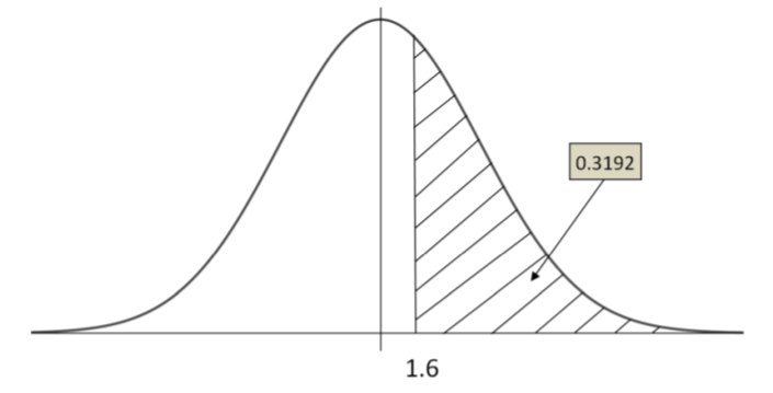
Example: Text messages

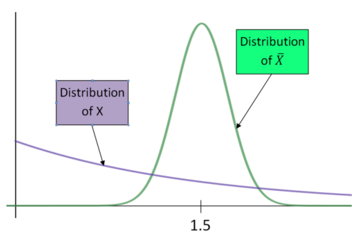
The waiting time until receiving a text message follows an exponential distribution with an expected waiting time of 1.5 minutes. Find the probability that the mean waiting time for the 50 text messages exceeds 1.6 minutes.

Solution

For the exponential distribution, the mean equals the standard deviation. Since the sample size is over 30, the distribution of \(\overline{X}\) will be normal, even though the distribution of \(X\) is heavily skewed.

\(\mu=1.6 \qquad \sigma=1.6 \qquad n=50\)

\(\begin{aligned}
P(\bar{X}>1.6) &=P\left(Z>\frac{(1.6-1.5)}{1.5 / \sqrt{50}}\right) \\
&=P(Z>0.47)\\&=0.3192
\end{aligned}\)