3.1: Measures of Central Tendency

Last updated
Save as PDF

Page ID: 20838

$ \newcommand{\vecs}[1]{\overset { \scriptstyle \rightharpoonup} {\mathbf{#1}} } $

$ \newcommand{\vecd}[1]{\overset{-\!-\!\rightharpoonup}{\vphantom{a}\smash {#1}}} $

$ \newcommand{\id}{\mathrm{id}}$ $ \newcommand{\Span}{\mathrm{span}}$

( \newcommand{\kernel}{\mathrm{null}\,}\) $ \newcommand{\range}{\mathrm{range}\,}$

$ \newcommand{\RealPart}{\mathrm{Re}}$ $ \newcommand{\ImaginaryPart}{\mathrm{Im}}$

$ \newcommand{\Argument}{\mathrm{Arg}}$ $ \newcommand{\norm}[1]{\| #1 \|}$

$ \newcommand{\inner}[2]{\langle #1, #2 \rangle}$

$ \newcommand{\Span}{\mathrm{span}}$

$ \newcommand{\id}{\mathrm{id}}$

$ \newcommand{\Span}{\mathrm{span}}$

$ \newcommand{\kernel}{\mathrm{null}\,}$

$ \newcommand{\range}{\mathrm{range}\,}$

$ \newcommand{\RealPart}{\mathrm{Re}}$

$ \newcommand{\ImaginaryPart}{\mathrm{Im}}$

$ \newcommand{\Argument}{\mathrm{Arg}}$

$ \newcommand{\norm}[1]{\| #1 \|}$

$ \newcommand{\inner}[2]{\langle #1, #2 \rangle}$

$ \newcommand{\Span}{\mathrm{span}}$ $ \newcommand{\AA}{\unicode[.8,0]{x212B}}$

$ \newcommand{\vectorA}[1]{\vec{#1}} % arrow$

$ \newcommand{\vectorAt}[1]{\vec{\text{#1}}} % arrow$

$ \newcommand{\vectorB}[1]{\overset { \scriptstyle \rightharpoonup} {\mathbf{#1}} } $

$ \newcommand{\vectorC}[1]{\textbf{#1}} $

$ \newcommand{\vectorD}[1]{\overrightarrow{#1}} $

$ \newcommand{\vectorDt}[1]{\overrightarrow{\text{#1}}} $

$ \newcommand{\vectE}[1]{\overset{-\!-\!\rightharpoonup}{\vphantom{a}\smash{\mathbf {#1}}}} $

$ \newcommand{\vecs}[1]{\overset { \scriptstyle \rightharpoonup} {\mathbf{#1}} } $

$ \newcommand{\vecd}[1]{\overset{-\!-\!\rightharpoonup}{\vphantom{a}\smash {#1}}} $

$\newcommand{\avec}{\mathbf a}$ $\newcommand{\bvec}{\mathbf b}$ $\newcommand{\cvec}{\mathbf c}$ $\newcommand{\dvec}{\mathbf d}$ $\newcommand{\dtil}{\widetilde{\mathbf d}}$ $\newcommand{\evec}{\mathbf e}$ $\newcommand{\fvec}{\mathbf f}$ $\newcommand{\nvec}{\mathbf n}$ $\newcommand{\pvec}{\mathbf p}$ $\newcommand{\qvec}{\mathbf q}$ $\newcommand{\svec}{\mathbf s}$ $\newcommand{\tvec}{\mathbf t}$ $\newcommand{\uvec}{\mathbf u}$ $\newcommand{\vvec}{\mathbf v}$ $\newcommand{\wvec}{\mathbf w}$ $\newcommand{\xvec}{\mathbf x}$ $\newcommand{\yvec}{\mathbf y}$ $\newcommand{\zvec}{\mathbf z}$ $\newcommand{\rvec}{\mathbf r}$ $\newcommand{\mvec}{\mathbf m}$ $\newcommand{\zerovec}{\mathbf 0}$ $\newcommand{\onevec}{\mathbf 1}$ $\newcommand{\real}{\mathbb R}$ $\newcommand{\twovec}[2]{\left[\begin{array}{r}#1 \\ #2 \end{array}\right]}$ $\newcommand{\ctwovec}[2]{\left[\begin{array}{c}#1 \\ #2 \end{array}\right]}$ $\newcommand{\threevec}[3]{\left[\begin{array}{r}#1 \\ #2 \\ #3 \end{array}\right]}$ $\newcommand{\cthreevec}[3]{\left[\begin{array}{c}#1 \\ #2 \\ #3 \end{array}\right]}$ $\newcommand{\fourvec}[4]{\left[\begin{array}{r}#1 \\ #2 \\ #3 \\ #4 \end{array}\right]}$ $\newcommand{\cfourvec}[4]{\left[\begin{array}{c}#1 \\ #2 \\ #3 \\ #4 \end{array}\right]}$ $\newcommand{\fivevec}[5]{\left[\begin{array}{r}#1 \\ #2 \\ #3 \\ #4 \\ #5 \\ \end{array}\right]}$ $\newcommand{\cfivevec}[5]{\left[\begin{array}{c}#1 \\ #2 \\ #3 \\ #4 \\ #5 \\ \end{array}\right]}$ $\newcommand{\mattwo}[4]{\left[\begin{array}{rr}#1 \amp #2 \\ #3 \amp #4 \\ \end{array}\right]}$ $\newcommand{\laspan}[1]{\text{Span}\{#1\}}$ $\newcommand{\bcal}{\cal B}$ $\newcommand{\ccal}{\cal C}$ $\newcommand{\scal}{\cal S}$ $\newcommand{\wcal}{\cal W}$ $\newcommand{\ecal}{\cal E}$ $\newcommand{\coords}[2]{\left\{#1\right\}_{#2}}$ $\newcommand{\gray}[1]{\color{gray}{#1}}$ $\newcommand{\lgray}[1]{\color{lightgray}{#1}}$ $\newcommand{\rank}{\operatorname{rank}}$ $\newcommand{\row}{\text{Row}}$ $\newcommand{\col}{\text{Col}}$ $\renewcommand{\row}{\text{Row}}$ $\newcommand{\nul}{\text{Nul}}$ $\newcommand{\var}{\text{Var}}$ $\newcommand{\corr}{\text{corr}}$ $\newcommand{\len}[1]{\left|#1\right|}$ $\newcommand{\bbar}{\overline{\bvec}}$ $\newcommand{\bhat}{\widehat{\bvec}}$ $\newcommand{\bperp}{\bvec^\perp}$ $\newcommand{\xhat}{\widehat{\xvec}}$ $\newcommand{\vhat}{\widehat{\vvec}}$ $\newcommand{\uhat}{\widehat{\uvec}}$ $\newcommand{\what}{\widehat{\wvec}}$ $\newcommand{\Sighat}{\widehat{\Sigma}}$ $\newcommand{\lt}{<}$ $\newcommand{\gt}{>}$ $\newcommand{\amp}{&}$ $\definecolor{fillinmathshade}{gray}{0.9}$

Let’s start this section with an example and a multiple choice question:

Example: Pizza delivery

Anthony’s Pizza, a Detroit based company, offers pizza delivery to its customers. A driver for Anthony’s Pizza will often make several deliveries on a single delivery run. A sample of 5 delivery runs by a driver showed the total number of pizzas delivered on each run:²³

2 2 5 9 12

What is the “average” number of pizzas sent out on a delivery run?

2 pizzas
5 pizzas
6 pizzas

Pick what you think is the answer and we will return to this example and discuss the answer at the end of this section.

Sample Mean

The sample mean is the arithmetic average of the data values. You simply add up all the numbers and divide by the sample size. The symbol $\bar{X}$ (pronounced X‐bar) refers to the sample mean.

Definition: Sample Mean

If $X_{1}, X_{2}, \cdots, X_{n}$ represents a sample of size $n$, then the sample mean is:

\[\bar{X}=\dfrac{X_{1}+X_{2}+\cdots+X_{n}}{n}=\dfrac{\sum X_{i}}{n} \nonumber\]

For the Example - Pizza delivery data, the sample mean is $\bar{X}=\dfrac{2+2+5+9+12}{5}=6$ pizzas (the middle value).

Sample Median

The sample median is the value that represents the exact middle of data, when the values are sorted from lowest to highest.

Procedure for finding the sample median

Sort the data values from lowest to highest.
If there is an odd number of values, the sample median is the middle value. \[\text { The median of }\{1,3,8,13,14\} \text { is } 8 \nonumber \]
If there is an even number of values, the sample median is the mean of the 2 middle values \[\text { The median of }\{1,3,8,10,13,14\} \text { is } \dfrac{8+10}{2}=9 \nonumber \]

Example: Pizza delivery

For the pizza delivery data {2, 2, 5, 9, 12}, the sample median is 5 pizzas (the middle value).

Example: Home prices in a single neighborhood

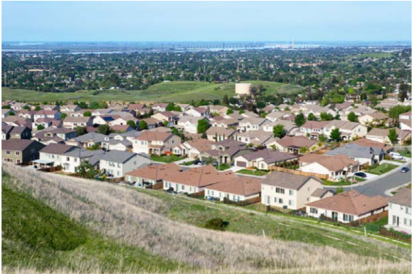
Here are the selling prices of 6 homes in the same neighborhood in Antioch, California²⁴:

$500,000 $550,000 $600,000 $700,000 $700,000 $1,950,000

The sample mean is $1,000,000 (add up the values and divide by 5).

The sample median is $650,000 ($600,000 plus $700,000 divided by 2).

Which of the two values is a better measure of the “average” home in this neighborhood?

Here the sample median is a better measure of center, because $650,000 better represents a typical home in this neighborhood. The mean is not a good measure of center here because the value of the outlier home, which costs $1,950,000. The median will never be affected by outliers because it is only location that matters when calculating the median.

Unlike the mean, the median (which is based on ranking instead of values), can be calculated for ordinal categorical data, but not for nominal data.

Example: Grades in a math class

In a community college algebra class, an instructor gave out the following grades to 40 students. Determine the median grade for the course.

The first step is to sort the grades from lowest to highest:

The middle values are both B’s, so the median grade is B.

Sample mode

The sample mode is the most frequently occurring value in the data. If there are multiple values that occur most frequently, then there are multiple modes in the data.

Example: Pizza delivery

For the pizza delivery data {2, 2, 5, 9, 12} , the sample mode is 2 pizzas because 2 occurs most frequently in the data.

Let's now return to the original question at the beginning of this section.

What is the “average” number of pizzas sent out on a delivery run?

2 pizzas
5 pizzas
6 pizzas

Since 2 is the mode, 5 is the median and 6 is the mean, practically speaking all 3 answers are examples of "averages". Lightbulb Books humorously calls these statistics "The Average Bears."²⁵

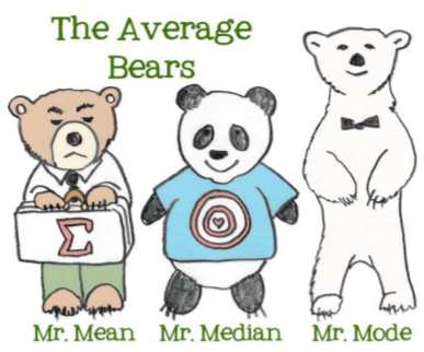
Many (including some Statistics texts) will automatically assume that average is the same as mean. In general life, people will use the terms mean and average interchangeably. But in Statistics, when we use the word "average", we mean a value that represents the center of the data. There are many statistics that represent the center of the data, including the mean, median and mode.

The mode can also be used for both nominal and ordinal categorical data.

Example: Nominal data ‐ Marital status

Let's return to the sample of 500 adults (aged 18 and over) from Santa Clara County taken from the year 2000 United States Census.

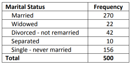
The mode for this data is value with the highest frequency, "Married."

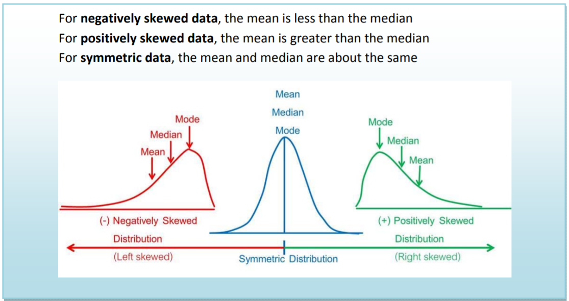
Using the mean and median to determine skewness

Skewness is a measure of how asymmetric the data vales are. Data can be positively skewed (stretched to the right), negatively skewed (stretched to the left) or symmetric (no skewness). Let’s now explore what effect skewness has on measures of center with several examples.

Example: Symmetric data – Heights of men

Here is a dot plot and summary statistics of the heights in inches of 1000 men, aged 30 years

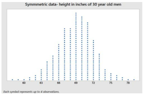
Sample mean = 68.98 inches

Sample median = 69 inches

Sample mode = 69 inches

The data values are evenly spread on the right and left of the peak. When data are symmetric, the mean, median and mode are about the same.

Example: Positively skewed data – Redwood trees

Here is a dot plot and summary statistics of the age of 1000 redwood trees sampled in California parks.

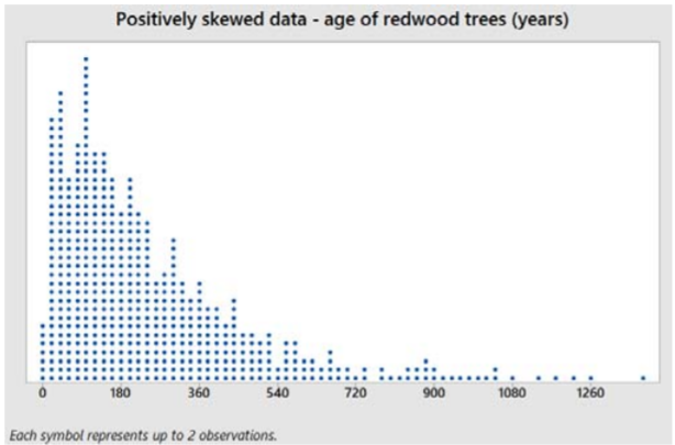
Sample mean = 237.48 years

Sample median = 180 years

Sample mode = 100 years

The data values are stretched to the right of center, causing the mean to be greater than the median. Also, the median will usually be greater than the mode for positively skewed data.

Example: Negatively skewed data – Exam grades

Here is a dot plot and summary statistics of the percentage grade of 1000 midterm exams given by a math instructor to algebra students.

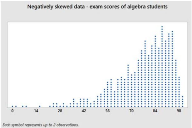
Sample mean = 76.21

Sample median = 80

Sample mode = 91

The data values are stretched to the left of center, causing the mean to be less than the median. Also, the median will usually be less than the mode for negatively skewed data.

Using the mean and median to find skewness in data²⁶

Example: Students browsing the web

From a prior example, this stem and leaf graph represents how much time 30 students spent on a web browser (on the Internet) in a 24 hour period. Data is rounded to the nearest minute.

\[\begin{array}{ll}
6 & 7 \\
7 & 18 \\
8 & 25677 \\
9 & 25799 \\
10 & 01233455789 \\
11 & 268 \\
12 & 245
\end{array} \nonumber \]

The sample median is 101.5 minutes, since the 15th observation is 101 and the 16th observation is 102.

Since the data is skewed negative, we would expect the sample mean to be less than the sample median.

Adding up the values and dividing by 30, we calculate that the sample mean is 96.6 minutes, consistent with data values that are negatively skewed.

Note that the mode is not helpful in this example since the sample size is small.

Search

Text Color

Text Size

Margin Size

Font Type

Sample Mean

Sample Median

Sample mode

Using the mean and median to determine skewness

Using the mean and median to find skewness in data26

Using the mean and median to find skewness in data²⁶