16.4: NHST in a Modern Context- Multiple Testing

So far we have discussed examples where we are interested in testing a single statistical hypothesis, and this is consistent with traditional science which often measured only a few variables at a time. However, in modern science we can often measure millions of variables per individual. For example, in genetic studies that quantify the entire genome, there may be many millions of measures per individual, and in brain imaging we often collect data from more than 100,000 locations in the brain at once. When standard hypothesis testing is applied in these contexts, bad things can happen unless we take appropriate care.

Let’s look at an example to see how this might work. There is great interest in understanding the genetic factors that can predispose individuals to major mental illnesses such as schizophrenia, because we know that about 80% of the variation between individuals in the presence of schizophrenia is due to genetic differences. The Human Genome Project and the ensuing revolution in genome science has provided tools to examine the many ways in which humans differ from one another in their genomes. One approach that has been used in recent years is known as a genome-wide association study (GWAS), in which the genome of each individual is characterized at one million or more places in their genome to determine which letters of the genetic code (which we call “variants”) they have at that location. After these have been determined, the researchers perform a statistical test at each location in the genome to determine whether people diagnosed with schizoprenia are more or less likely to have one specific variant at that location.

Let’s imagine what would happen if the researchers simply asked whether the test was significant at p<.05 at each location, when in fact there is no true effect at any of the locations. To do this, we generate a large number of simulated t values from a null distribution, and ask how many of them are significant at p<.05. Let’s do this many times, and each time count up how many of the tests come out as significant (see Figure 16.8).

## [1] "corrected familywise error rate: 0.036"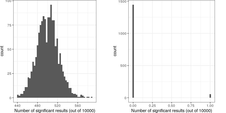

Figure 16.8: Left: A histogram of the number of significant results in each set of 1 million statistical tests, when there is in fact no true effect. Right: A histogram of the number of significant results across all simulation runs after applying the Bonferroni correction for multiple tests.

This shows that about 5% of all of the tests were significant in each run, meaning that if we were to use p < .05 as our threshold for statistical significance, then even if there were no truly significant relationships present, we would still “find” about 500 genes that were seemingly significant (the expected number of significant results is simply $n * \alpha$). That is because while we controlled for the error per test, we didn’t control the familywise error, or the error across all of the tests, which is what we really want to control if we are going to be looking at the results from a large number of tests. Using p<.05, our familywise error rate in the above example is one – that is, we are pretty much guaranteed to make at least one error in any particular study.

A simple way to control for the familywise error is to divide the alpha level by the number of tests; this is known as the Bonferroni correction, named after the Italian statistician Carlo Bonferroni. Using the data from our example above, we see in Figure ?? that only about 5 percent of studies show any significant results using the corrected alpha level of 0.000005 instead of the nominal level of .05. We have effectively controlled the familywise error, such that the probability of making any errors in our study is controlled at right around .05.