11.4: Independent Sampling – Comparing Two Population Variances or Standard Deviations
- Page ID
- 20916

Sometimes we want to test if two populations have the same spread or variation, as measured by variance or standard deviation. This may be a test on its own or a way of checking assumptions when deciding between two different models (e.g.: pooled variance \(t\)‐test vs. unequal variance \(t\)‐test). We will now explore testing for a difference in variance between two independent samples.
The \(\mathbf{F}\) distribution is a family of distributions related to the Normal Distribution. There are two different degrees of freedom, usually represented as numerator (\(\mathrm{df}_{\text {num}}\)) and denominator (\(\mathrm{df}_{\text {den}}\)). Also, since the F represents squared data, the inference will be about the variance rather than the about the standard deviation.
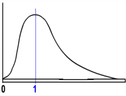
- It is positively skewed
- It is non‐negative
- There are 2 different degrees of freedom (\(\mathrm{df}_{\text {num}}\), \(\mathrm{df}_{\text {den}}\))
- When the degrees of freedom change, a new distribution is created
- The expected value is 1.
\(\mathbf{F}\) test for equality of variances
Suppose we wanted to test the Null Hypothesis that two population standard deviations are equal, \(H_o: \sigma_{1}=\sigma_{2}\). This is equivalent to testing that the population variances are equal: \(\sigma_{1}^{2}=\sigma_{2}^{2}\). We will now instead write these as an equivalent ratio: \(H_o: \dfrac{\sigma_{1}^{2}}{\sigma_{2}^{2}}=1\) or \(H_o: \dfrac{\sigma_{2}^{2}}{\sigma_{2}^{1}}=1\).
This is the logic behind the \(\mathbf{F}\) test; if two population variances are equal, then the ratio of sample variances from each population will have \(\mathbf{F}\) distribution. \(\mathbf{F}\) will always be an upper tailed test in practice, so the larger variance goes in the numerator. The test statistics are summarized in the table.
| Hypotheses | Test Statistic |
|---|---|
| \(\begin{aligned} &H_{o}: \sigma_{1} \geq \sigma_{2} \\ &H_{a}: \sigma_{1}<\sigma_{2} \end{aligned}\) |
\(\mathbf{F}=\dfrac{s_{2}^{2}}{s_{1}^{2}}\) use \(\alpha\) table |
| \(\begin{aligned} &H_{o}: \sigma_{1} \leq \sigma_{2} \\ &H_{a}: \sigma_{1}>\sigma_{2} \end{aligned}\) |
\(\mathbf{F}=\dfrac{s_{1}^{2}}{s_{2}^{2}}\) use \(\alpha\) table |
| \(\begin{aligned} &H_{o}: \sigma_{1}=\sigma_{2} \\ &H_{a}: \sigma_{1} \neq \sigma_{2} \end{aligned}\) |
\(\mathbf{F}=\dfrac{\max \left(s_{1}^{2}, s_{2}^{2}\right)}{\min \left(s_{1}^{2}, s_{2}^{2}\right)}\) use \(\alpha/2\) table |
Example: Variation in stocks

A stockbroker at a brokerage firm, reported that the mean rate of return on a sample of 10 software stocks (population 1)was 12.6 percent with a standard deviation of 4.9 percent. The mean rate of return on a sample of 8 utility stocks (population 2) was 10.9, percent with a standard deviation of 3.5 percent. At the .05 significance level, can the broker conclude that there is more variation in the software stocks?
Solution
Design
Research Hypotheses:
\(H_o: \sigma_{1} \leq \sigma_{2}\) (Software stocks do not have more variation)
\(H_a: \sigma_{1} > \sigma_{2}\) (Software stocks do have more variation)
Model will be \(\mathbf{F}\) test for variances and the test statistic from the table will be \(\mathbf{F}=\dfrac{s_{1}^{2}}{s_{2}^{2}}\). The degrees of freedom for numerator will be \(n_{1}-1=9\), and the degrees of freedom for denominator will be \(n_{2}-1=7\). The test will be run at a level of significance (\(\alpha\)) of 5%. Critical Value for \(\mathbf{F}\) with \(\mathrm{df}_{\text {num}}=9\) and \(\mathrm{df}_{\text {den}}=7\) is 3.68. Reject \(H_o\) if \(\mathbf{F}\) >3.68.
Data/Results
\(\mathbf{F}=4.9^{2} / 3.5^{2}=1.96\), which is less than critical value, so Fail to Reject \(H_o\).
Conclusion
There is insufficient evidence to claim more variation in the software stock.
Example: Testing model assumptions
When comparing two means from independent samples, you have a choice between the more powerful pooled variance \(t\)‐test (assumption is \(\sigma_{1}^{2}=\sigma_{2}^{2}\)) or the weaker unequal variance \(t\)‐test (assumption is \(\sigma_{1}^{2} \neq \sigma_{2}^{2}\). We can now design a hypothesis test to help us choose the appropriate model. Let us revisit the example of comparing the MPG for import and domestic compact cars. Consider this example a "test before the main test" to help choose the correct model for comparing means.
Solution
Design
Research Hypotheses:
\(H_o: \sigma_{1} = \sigma_{2}\) (choose the pooled variance \(t\)‐test to compare means)
\(H_a: \sigma_{1} \neq \sigma_{2}\) (choose the unequal variance \(t\)‐test to compare means)
Model will be \(\mathbf{F}\) test for variances, and the test statistic from the table will be \(\mathbf{F}=\dfrac{s_{1}^{2}}{s_{2}^{2}}\) (\(s_1\) is larger). The degrees of freedom for numerator will be \(n_{1}-1=11\) and the degrees of freedom for denominator will be \(n_2‐1=14\). The test will be run at a level of significance (\(\alpha\)) of 10%, but use the \(\alpha\)=.05 table for a two‐tailed test. Critical Value for \(\mathbf{F}\) with \(\mathrm{df}_{\text {num}}=11\) and \(\mathrm{df}_{\text {den}}=14\) is 2.57. Reject \(H_o\) if \(\mathbf{F}\) >2.57.
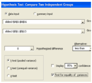
We will also run this test the \(p\)‐value way in Megastat.
Data/Results
\(\mathbf{F}=14.894 / 4.654=3.20\), which is more than critical value; Reject \(H_o\).
Also \(p\)‐value = 0.0438 < 0.10, which also makes the result significant.
Conclusion
Do not assume equal variances and run the unequal variance \(t\)‐test to compare population means
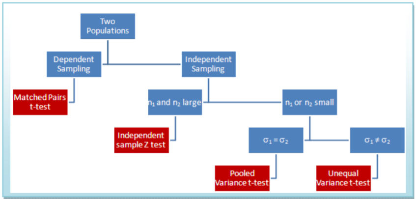
In Summary
This flowchart summarizes which of the four models to choose when comparing two population means. In addition, you can use the \(\mathbf{F}\)‐test for equality of variances to make the decision between the pool variance \(t\)‐test and the unequal variance \(t\)‐test.