
8: Chi Square
- Page ID
- 5428

\( \newcommand{\vecs}[1]{\overset { \scriptstyle \rightharpoonup} {\mathbf{#1}} } \)
\( \newcommand{\vecd}[1]{\overset{-\!-\!\rightharpoonup}{\vphantom{a}\smash {#1}}} \)
\( \newcommand{\dsum}{\displaystyle\sum\limits} \)
\( \newcommand{\dint}{\displaystyle\int\limits} \)
\( \newcommand{\dlim}{\displaystyle\lim\limits} \)
\( \newcommand{\id}{\mathrm{id}}\) \( \newcommand{\Span}{\mathrm{span}}\)
( \newcommand{\kernel}{\mathrm{null}\,}\) \( \newcommand{\range}{\mathrm{range}\,}\)
\( \newcommand{\RealPart}{\mathrm{Re}}\) \( \newcommand{\ImaginaryPart}{\mathrm{Im}}\)
\( \newcommand{\Argument}{\mathrm{Arg}}\) \( \newcommand{\norm}[1]{\| #1 \|}\)
\( \newcommand{\inner}[2]{\langle #1, #2 \rangle}\)
\( \newcommand{\Span}{\mathrm{span}}\)
\( \newcommand{\id}{\mathrm{id}}\)
\( \newcommand{\Span}{\mathrm{span}}\)
\( \newcommand{\kernel}{\mathrm{null}\,}\)
\( \newcommand{\range}{\mathrm{range}\,}\)
\( \newcommand{\RealPart}{\mathrm{Re}}\)
\( \newcommand{\ImaginaryPart}{\mathrm{Im}}\)
\( \newcommand{\Argument}{\mathrm{Arg}}\)
\( \newcommand{\norm}[1]{\| #1 \|}\)
\( \newcommand{\inner}[2]{\langle #1, #2 \rangle}\)
\( \newcommand{\Span}{\mathrm{span}}\) \( \newcommand{\AA}{\unicode[.8,0]{x212B}}\)
\( \newcommand{\vectorA}[1]{\vec{#1}} % arrow\)
\( \newcommand{\vectorAt}[1]{\vec{\text{#1}}} % arrow\)
\( \newcommand{\vectorB}[1]{\overset { \scriptstyle \rightharpoonup} {\mathbf{#1}} } \)
\( \newcommand{\vectorC}[1]{\textbf{#1}} \)
\( \newcommand{\vectorD}[1]{\overrightarrow{#1}} \)
\( \newcommand{\vectorDt}[1]{\overrightarrow{\text{#1}}} \)
\( \newcommand{\vectE}[1]{\overset{-\!-\!\rightharpoonup}{\vphantom{a}\smash{\mathbf {#1}}}} \)
\( \newcommand{\vecs}[1]{\overset { \scriptstyle \rightharpoonup} {\mathbf{#1}} } \)
\(\newcommand{\longvect}{\overrightarrow}\)
\( \newcommand{\vecd}[1]{\overset{-\!-\!\rightharpoonup}{\vphantom{a}\smash {#1}}} \)
\(\newcommand{\avec}{\mathbf a}\) \(\newcommand{\bvec}{\mathbf b}\) \(\newcommand{\cvec}{\mathbf c}\) \(\newcommand{\dvec}{\mathbf d}\) \(\newcommand{\dtil}{\widetilde{\mathbf d}}\) \(\newcommand{\evec}{\mathbf e}\) \(\newcommand{\fvec}{\mathbf f}\) \(\newcommand{\nvec}{\mathbf n}\) \(\newcommand{\pvec}{\mathbf p}\) \(\newcommand{\qvec}{\mathbf q}\) \(\newcommand{\svec}{\mathbf s}\) \(\newcommand{\tvec}{\mathbf t}\) \(\newcommand{\uvec}{\mathbf u}\) \(\newcommand{\vvec}{\mathbf v}\) \(\newcommand{\wvec}{\mathbf w}\) \(\newcommand{\xvec}{\mathbf x}\) \(\newcommand{\yvec}{\mathbf y}\) \(\newcommand{\zvec}{\mathbf z}\) \(\newcommand{\rvec}{\mathbf r}\) \(\newcommand{\mvec}{\mathbf m}\) \(\newcommand{\zerovec}{\mathbf 0}\) \(\newcommand{\onevec}{\mathbf 1}\) \(\newcommand{\real}{\mathbb R}\) \(\newcommand{\twovec}[2]{\left[\begin{array}{r}#1 \\ #2 \end{array}\right]}\) \(\newcommand{\ctwovec}[2]{\left[\begin{array}{c}#1 \\ #2 \end{array}\right]}\) \(\newcommand{\threevec}[3]{\left[\begin{array}{r}#1 \\ #2 \\ #3 \end{array}\right]}\) \(\newcommand{\cthreevec}[3]{\left[\begin{array}{c}#1 \\ #2 \\ #3 \end{array}\right]}\) \(\newcommand{\fourvec}[4]{\left[\begin{array}{r}#1 \\ #2 \\ #3 \\ #4 \end{array}\right]}\) \(\newcommand{\cfourvec}[4]{\left[\begin{array}{c}#1 \\ #2 \\ #3 \\ #4 \end{array}\right]}\) \(\newcommand{\fivevec}[5]{\left[\begin{array}{r}#1 \\ #2 \\ #3 \\ #4 \\ #5 \\ \end{array}\right]}\) \(\newcommand{\cfivevec}[5]{\left[\begin{array}{c}#1 \\ #2 \\ #3 \\ #4 \\ #5 \\ \end{array}\right]}\) \(\newcommand{\mattwo}[4]{\left[\begin{array}{rr}#1 \amp #2 \\ #3 \amp #4 \\ \end{array}\right]}\) \(\newcommand{\laspan}[1]{\text{Span}\{#1\}}\) \(\newcommand{\bcal}{\cal B}\) \(\newcommand{\ccal}{\cal C}\) \(\newcommand{\scal}{\cal S}\) \(\newcommand{\wcal}{\cal W}\) \(\newcommand{\ecal}{\cal E}\) \(\newcommand{\coords}[2]{\left\{#1\right\}_{#2}}\) \(\newcommand{\gray}[1]{\color{gray}{#1}}\) \(\newcommand{\lgray}[1]{\color{lightgray}{#1}}\) \(\newcommand{\rank}{\operatorname{rank}}\) \(\newcommand{\row}{\text{Row}}\) \(\newcommand{\col}{\text{Col}}\) \(\renewcommand{\row}{\text{Row}}\) \(\newcommand{\nul}{\text{Nul}}\) \(\newcommand{\var}{\text{Var}}\) \(\newcommand{\corr}{\text{corr}}\) \(\newcommand{\len}[1]{\left|#1\right|}\) \(\newcommand{\bbar}{\overline{\bvec}}\) \(\newcommand{\bhat}{\widehat{\bvec}}\) \(\newcommand{\bperp}{\bvec^\perp}\) \(\newcommand{\xhat}{\widehat{\xvec}}\) \(\newcommand{\vhat}{\widehat{\vvec}}\) \(\newcommand{\uhat}{\widehat{\uvec}}\) \(\newcommand{\what}{\widehat{\wvec}}\) \(\newcommand{\Sighat}{\widehat{\Sigma}}\) \(\newcommand{\lt}{<}\) \(\newcommand{\gt}{>}\) \(\newcommand{\amp}{&}\) \(\definecolor{fillinmathshade}{gray}{0.9}\)In chapter 5, the inferential theory for categorical data was developed based upon the binomial distribution. Recall that the binomial distribution shows the probability of the possible number of successes in a sample of size n when there were only two possible independent outcomes, success and failure. What happens if there are more than two possible outcomes however?
Consider the following three questions.
- Does the TI 84 calculator generate equal numbers of 0-9 when using the random integer generator?
- Doing something about climate change has been a challenge for humanity. The website Edge.Org had one proposal put forth by Lee Smolin, a physicist with the Perimeter Institute and author of book Time Reborn.(www.edge.org/conversation/del...ooperation/#rc Nov 30, 2013.) The essence of the proposal is that a carbon tax should be placed on all carbon that is used but instead of the money going to the government it goes to individual climate retirement accounts. Each person would have such an account. Each account would have two categories of possible investments that an individual could choose. Category A investments would be in things that will mitigate climate change (e.g. solar, wind, etc). Category B investments would be in things that might do well if climate change does not happen (e.g. utilities that burn coal, coastal real estate developments and car companies that do not produce fuel efficient or electric cars). Is there a correlation between a person’s opinion about climate change and their choice of investment?
- Hurricanes are classified as category 1,2,3,4,5. Is the distribution of hurricanes in the years 1951- 2000 different than it was in 1901-1950?
Before an analysis can be done, it is necessary to understand the type of data that is gathered for each of these questions.
In question 1, the data that will be gathered are the numbers 0 though 9. While numbers are typically considered quantitative, in this case we simply want to know if the calculator produces each specific number. Therefore, this is actually about the frequency with which these numbers are produced. If the process used by the calculator is sufficiently random, then the frequencies for all the numbers should be equal if a large enough sample is taken. So, in spite of appearing to be quantitative data, this is actually categorical data, with 10 different categories and the data being that a number was selected.
In question 2, imagine a two-question survey in which people are asked:
- Do you believe climate change is happening because humans have been using carbon sources that lead to an increase in greenhouse gases? Yes No
- Which of the following most closely represents the choice you would make for your individual climate retirement account investments? Category A Category B
For this question, there is one population. Each person that takes the survey would provide two answers. The objective is to determine if there is a correlation between their climate change opinion and their investment choice. An alternate way of saying this is that the two variables are either independent of each other, which means that one response does not affect the other, or they are not independent which means that climate change opinion and investment strategy are related.
In question 3, there are two populations. The first population is hurricanes in 1901-50 and the second population is hurricanes in 1951-2000. There are 5 categories of hurricanes and the goal is to see if the distribution of hurricanes in these categories is the same or different.
The problems fit one of the following classes of problems, in order: goodness of fit, test for independence, and test for homogeneity. The use of these problems and their hypotheses are shown below.
- Goodness of Fit
The goodness of fit test is used when a categorical random variable with more than two levels has an expected distribution.
\(H_0\): The distribution is the same as expected
\(H_1\): The distribution is different than expected - Test for Independence
The test for independence is used when there are two categorical random variables for the same unit (or person) and the objective is to determine a correlation between them.
\(H_0\): The two random variables are independent (no correlation)
\(H_1\): The two random variables are not independent (correlation)
If the data are significant, than knowledge of the value of one of the random variables increases the probability of knowing the value of the other random variable compared to chance. - Test for Homogeneity
The test for homogeneity is used when there are samples taken from two (or more) populations with the objective of determining if the distribution of one random variable is similar or different in the two populations.
\(H_0\): The two populations are homogeneous
\(H_1\): The two populations are not homogeneousSince all of the problems have data that can be counted exactly one time, the strategy is to determine how the distribution of counts differs from the expected distribution. The analysis of all these problems uses the same test statistic formula called \(chi ^2\)(Chi Square).
\[\chi^2 = \sum \dfrac{(O - E)^2}{E}\]
The distribution that is used for testing the hypotheses is the set of \(chi ^2\) distributions. These distributions are positively skewed. They cannot be negative. Each distribution is based on the number of degrees of freedom. Unlike the t distributions in which degrees of freedom were based on the sample size, in the case of \(chi ^2\), the degrees of freedom are based on the number of levels of the random variable(s).
The following distributions show 10,000 samples of size n = 100 in which the \(chi ^2\) test statistics calculated and graphed. The numbers of degrees of freedom in these four graphs are 1,2,5, and 9.
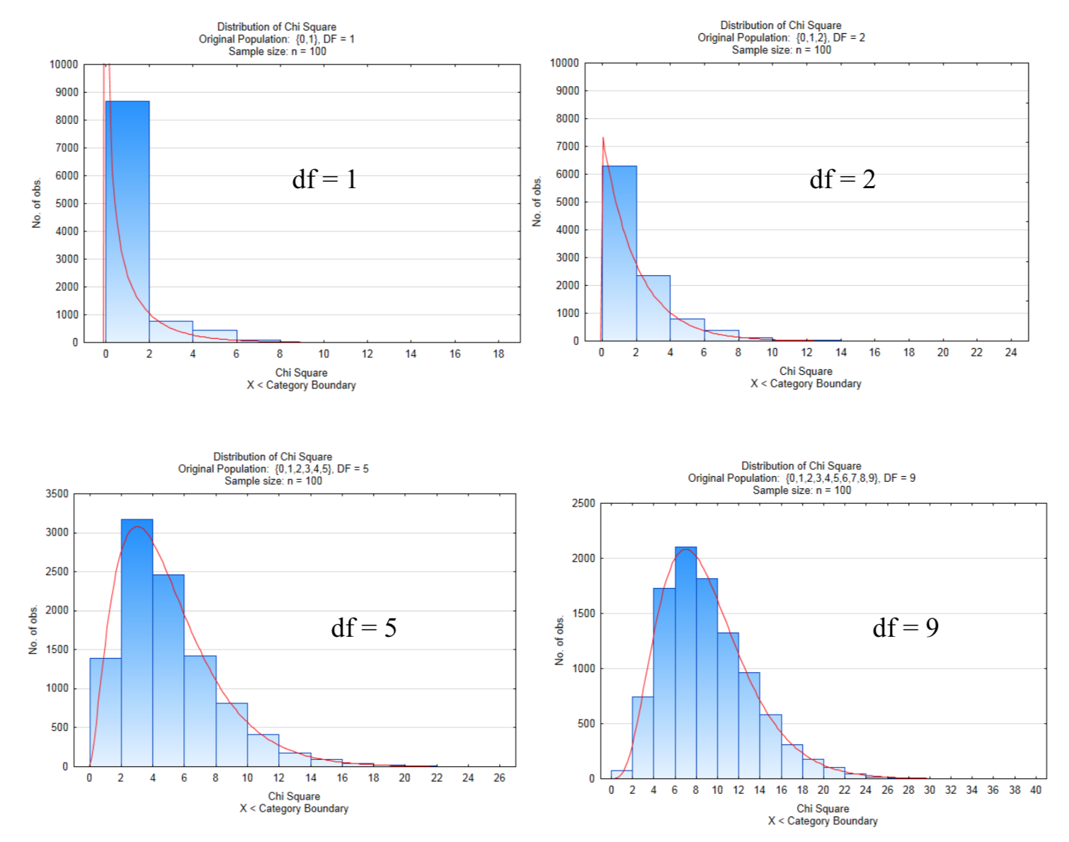
Notice how the Chi Square distribution becomes less skewed and is approaching a normal distribution as the number of degrees of freedom increase. An increase in the number of degrees of freedom corresponds to an increase in the number of levels of the explanatory factor. The way in which degrees of freedom are found is different for the goodness of fit test compared to the test for independence and test for homogeneity. Each method will be explained in turn.
Goodness of Fit Test
1. Does the TI 84 calculator generate equal numbers of 0-9 when using the random integer generator?
In this experiment, 12 numbers between 1 and 100 were randomly generated by the TI 84 calculator. These 12 numbers were used as seed values. After seeding the calculator with each number, 10 new numbers between 0 and 9 were randomly generated using the randint function on the calculator. Thus, a total of 120 numbers between 0 and 9 were produced. The frequency of these numbers is shown in the table below.
| 0 | 1 | 2 | 3 | 4 | 5 | 6 | 7 | 8 | 9 |
| 15 | 11 | 12 | 14 | 10 | 14 | 10 | 11 | 14 | 9 |
The hypotheses to be tested are:
\(H_0\): The observed cell frequency equals the expected cell frequency for all cells
\(H_1\): The observed cell frequency does not equal the expected cell frequency for at least one cell. Use a 0.05 level of significance
This can be represented symbolically as
\(H_0\): \(o_1 = \epsilon_1\) for all cells
\(H_1\): \(o_1 \ne \epsilon_1\) for at least one cell
where ο is the lower case Greek letter omicron that represents the observed cell frequency in the underlying population and ε is the lower case Greek letter epsilon that represents the expected cell frequency. The expected cell frequency should always be 5 or higher. If it isn’t, cells should be regrouped.
The table above shows the observed frequencies, but what are the expected frequencies? In theory, if the process is truly random, then each number would occur with the same frequency if the sampling were to be done a very large number of times. If this is the case, then in a sample of size 120, with 10 possible alternatives, the expected number of frequencies for each alternative should be 12. From the table, we see that most frequencies are not 12, but what is needed is a way to determine if the amount of variation that exists is enough to suggest that the observed frequencies do not equal the expected frequencies. Such a conclusion would imply the calculator does not produce a truly random set of numbers. The strategy is to find \(\chi^2\) and then use the appropriate \(\chi^2\) distribution to find the p-value. One way to find \(\chi^2 = \sum \dfrac{(O - E)^2}{E}\) is with a table.
| Observed | Expected | O - E | \((O - E)^2\) | \(\dfrac{(O - E)^2}{E}\) |
|---|---|---|---|---|
| 15 | 12 | 3 | 9 | \(\dfrac{9}{12}\) |
| 11 | 12 | -1 | 1 | \(\dfrac{1}{12}\) |
| 12 | 12 | 0 | 0 | \(\dfrac{0}{12}\) |
| 14 | 12 | 2 | 4 | \(\dfrac{4}{12}\) |
| 10 | 12 | -2 | 4 | \(\dfrac{4}{12}\) |
| 14 | 12 | 2 | 4 | \(\dfrac{4}{12}\) |
| 10 | 12 | -2 | 4 | \(\dfrac{4}{12}\) |
| 11 | 12 | -1 | 1 | \(\dfrac{1}{12}\) |
| 14 | 12 | 2 | 4 | \(\dfrac{4}{12}\) |
| 9 | 12 | -3 | 9 | \(\dfrac{9}{12}\) |
| \(\chi^2 = \dfrac{40}{12} = 3.33\) |
If r represents the number of rows, then the number of degrees of freedom in a goodness of fit test is:
df = r – 1.
For this Goodness of fit test, there are 10 rows of data. Consequently there are 9 degrees of freedom.
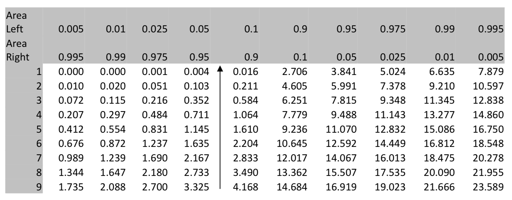
The p-value for \(\chi^2\) can be found using the table of the Chi Square Distributions at the end of this chapter or your calculator.
The Chi-Square Distributions can also be used to find the p-value. Using the table below, find the degrees of freedom in the left column, locate the \(\chi^2\) value in the row, then move to the row that shows the area to the right and use an inequality sign to show the p-value. If the p-value isgreater than \(\alpha\), then use the greater than symbol. If it is less than α, use the less than symbol, but in either case, use as much precision as possible. For example, if α is 0.05 but the area to the right is lessthan 0.025, then p < 0.025 is preferred over p < 0.05.
In this example, \(\chi^2\) = 3.33, there are 9 degrees of freedom, so the p-value > 0.9.
\(\chi^2 = 3.33\)
Using \(\chi^2\) cdf (low, high, df) in the TI 84 calculator results in \(\chi^2\) cdf (3.33, 1E99,9) = 0.9496.
Since this p-value is clearly higher than 0.05, the conclusion can be written:
At the 5% level of significance, the observed cell values are not significantly different than the expected cell values (\(\chi^2\) = 3.33, p = 0.9496, df=9). The TI84 calculator appears to produce a good set of random integers.
In the case of the calculator, if it is random in generating numbers, we would expect the same number of values in each category. That is, we would expect to get the same number of 0s, 1s, 2s, etc. Since the sample consisted of 120 trials with 10 possibilities for each outcome, the expected value is 12 because 120 divided by 10 is 12. But what happens if the expected outcome is not the same in all cases?
In the fall of 2013, our college was made up of 54% Caucasian, 14% Hispanic/Latino, 11% African American, 10% Asian/Pacific Islander, 1% Native American, 3% international, and 7% other. If we wanted to determine if the racial/ethnic distribution of statistics students is different than of the entire school, we could take a survey of statistics students to obtain the observed data. The table below contains hypothetical observed data. Since there are 300 students in the sample and based on college enrollment, 54% of the student body is white, then the expected number of students in the class who are white is found by multiplying 300 times 0.54. The same approach is taken for each race. This is shown in the table. Notice the total in the expected column is the same as in the observed column.
| Race/Ethnicity | Observed | Expected |
|---|---|---|
| Caucasian/white (54%) | 154 | 0.54(300) = 162 |
| Hispanic/Latino (14%) | 48 | 0.14(300) = 42 |
| African American/Black (11%) | 36 | 0.11(300) = 33 |
| Asian/Pacific Islander (10%) | 35 | 0.10(300) = 30 |
| Native American (1%) | 6 | 0.01(300) = 3 |
| International (3%) | 9 | 0.03(300) = 9 |
| Other (7%) | 12 | 0.07(300) = 21 |
| Total | 300 | Total 300 |
The remainder of the goodness of fit test is done the same as with the calculator example and will not be demonstrated here.
Chi Square Test for Independence
The Chi Square Test for Independence is used when a researcher wants to determine a relationship between two categorical random variables collected on the same unit (or person). Sample questions include:
- Is there a relationship between a person’s religious affiliation and their political party preference?
- Is there a relationship between a person’s willingness to eat genetically engineered food and their willingness to use genetically engineered medicine?
- Is there a relationship between the field of study for a college graduate and their ability to think critically?
- Is there a relationship between the quality of sleep a person gets and their attitude during the next day?
As an example, we will learn the mechanics of the test for independence using the hypothetical example of responses to the two questions about climate change and investments.
- Do you believe climate change is happening because humans have been using carbon sources that lead to an increase in greenhouse gases? Yes No
- Which of the following most closely represents the choice you would make for your individual climate retirement account investments? Category A Category B
Category A – solar, wind Category B – Coal, ocean side development
\(H_0\): The two random variables are independent (no correlation)
\(H_1\): The two random variables are not independent (correlation)
This can also be represented symbolically as
\(H_0: o_1 = \epsilon_1\) for all cells
\(H_1: o_1 \ne \epsilon_1\) for at least one cell
where \(o\) is the lower case Greek letter omicron that represents the observed cell frequency in the underlying population and \(\epsilon\) is the lower case Greek letter epsilon that represents the expected cell frequency. The expected cell frequency should always be 5 or higher. If it isn’t, cells should be regrouped.
Use a level of significance of 0.05.
Because this will be done with pretend data, it will be useful to do it twice, producing opposite conclusions each time.
The data will be presented in a 2 x 2 contingency table.
| Version 1 Observed |
Yes - humans contribute to clime change | No - humans do not contribute to climate change | Totals |
| Category A Investments (wind, solar) | 56 | 54 | |
| Category B Investments (coal, ocean shore developments) | 47 | 43 | |
| Total |
The test for independence uses the same formula as the goodness of fit test. \(\chi^2 = \sum \dfrac{(O - E)^2}{E}\). Unlike that test however, there is no clear indication of what the expected values are. Instead they must be calculated, which is a four-step process.
Step 1, Find the row and column totals and the grand total.
| Version 1 Observed |
Yes - humans contribute to clime change | No - humans do not contribute to climate change | Totals |
| Category A Investments (wind, solar) | 56 | 54 | 110 |
| Category B Investments (coal, ocean shore developments) | 47 | 43 | 90 |
| Total | 103 | 97 | 200 |
Step 2. Create a new table for the expected values. The reasoning process for calculating the expected values is to first consider the proportion of all the values that fall in each column. In the first column there are 103 values out of 200 which is \(\dfrac{}{} = 0.515\). In the second column there are 97 out of 200 values (0.485). Since 51.5% of the values are in the first column, then it would be expected that 51.5% of the first row’s values would also be in the first column. Thus, 0.515(110) gives an expected value of 56.65. Likewise, 0.485(90) will produce the expected value of 43.65 for the last cell. As a formula, this can be expressed as
\[\dfrac{Column\ Total}{Grand\ Total} \cdot Row\ Total\]
| Version 1 Observed |
Yes - humans contribute to clime change | No - humans do not contribute to climate change | Totals |
| Category A Investments (wind, solar) | \(\dfrac{103}{200} \cdot 110 = 56.65\) | \(\dfrac{97}{200} \cdot 110 = 53.35\) | 110 |
| Category B Investments (coal, ocean shore developments) | \(\dfrac{103}{200} \cdot 90 = 46.35\) | \(\dfrac{97}{200} \cdot 110 = 43.65\) | 90 |
| Total | 103 | 97 | 200 |
Step 3. Use a table similar to the one used in the Goodness of Fit test to calculate Chi Square.
| Observed | Expected | \(O - E\) | \((O - E)^2\) | \(\dfrac{(O - E)^2}{E}\) |
| 56 | 56.65 | -0.65 | 0.4225 | 0.0075 |
| 54 | 53.35 | 0.65 | 0.4225 | 0.0079 |
| 47 | 46.35 | 0.65 | 0.4225 | 0.0091 |
| 43 | 43.65 | -0.65 | 0.4225 | 0.0097 |
| \(\chi^2 = 0.0342\) |
Step 4. Determine the Degrees of Freedom and find the p-value
If R is the number of Rows in the contingency Table and C is the number of columns in the contingency table, then the number of degrees of freedom for the test for independence is found as
df = (R - 1)(C - 1).
For a 2 x 2 contingency table such as in this problem, there is only 1 degree of freedom because (2-1)(2-1) = 1.
The p-value for \(\chi^2\) can be found using the table or your calculator.
In the table we locate 0.034 in the row with 1 degree of freedom, then move up to the row for the area to the right. Since the area to the right is greater than 0.05, but more specifically it is greater than 0.1, the p-value is written as p > 0.1.
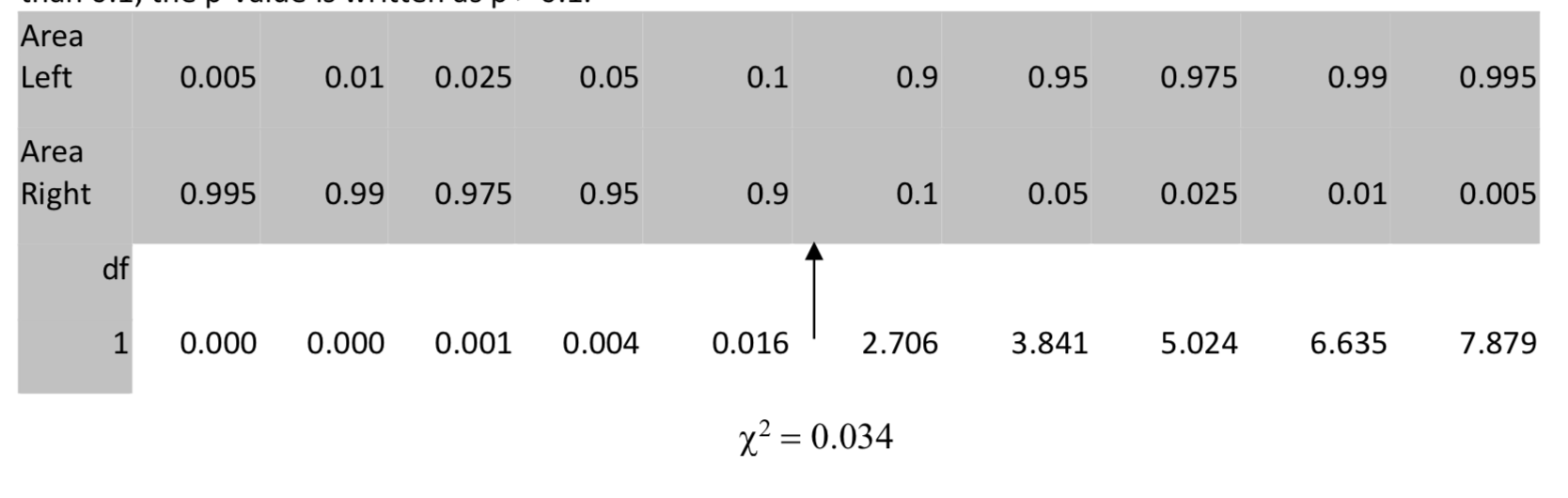
On your calculator, use \(\chi^2\) cdf (low, high, df) . In this case, \(\chi^2\) cdf (0.0342, 1E99, 1) = 0.853.
Since the data are not significant, we conclude that people’s investment strategy is independent of their opinion about human contributions to climate change.
Version 2 of this problem uses the following contingency table.
| Version 2 Observed |
Yes - humans contribute to clime change | No - humans do not contribute to climate change | Totals |
| Category A Investments (wind, solar) | 80 | 30 | |
| Category B Investments (coal, ocean shore developments) | 30 | 60 | |
| Total |
This time, the entire problem will be calculated using the TI 84 calculator instead of building the tables that were used in Version 1.
Step 1. Matrix
Step 2. Make 1:[A] into a 2 x 2 matrix by selecting Edit Enter then modify the R x C as necessary. Step 3. Enter the frequencies as they are shown in the table.
Step 4. STAT TESTS \(\chi^2\) − Test
Observed:[A]
Expected:[B] (you do not need to create the Expected matrix, the calculator will for you.)
Select Calculate to see the results:
\(\chi^2\) = 31.03764922
p=2.5307155E-8
df=1
In this case, the data are significant. This means that there is a correlation between each person’s opinion about human contributions to climate change and their choice of investments. Remember that correlation is not causation.
Chi Square Test for Homogeneity
The third and final problem is about the classification of hurricanes in two different decades, 1901-50 and 1951-2000. One theory about climate change is that hurricanes could get worse. be worked using tables.
Hurricanes are classified by the Saffir-Simpson Hurricane Wind Scale.2
Category 1 Sustained Winds 74-95 mph
Category 2 Sustained Winds 96-110 mph
Category 3 Sustained Winds 111-129 mph
Category 4 Sustained Winds 130-156 mph
Category 5 Sustained Winds 157 or higher.
Category 3, 4, and 5 hurricanes are considered major.
This problem will
The population of interest is the distribution of hurricanes for the prevailing climate conditions at the time. The hypotheses being tested are
\(H_0\): The distributions are homogeneous
\(H_1\): The distributions are not homogeneous
This can also be represented symbolically as
\(H_0: o_1 = \epsilon_1\) for all cells
\(H_1: o_1 \ne \epsilon_1\) for at least one cell
where \(o\) is the lower case Greek letter omicron that represents the observed cell frequency in the underlying population and \(\epsilon\) is the lower case Greek letter epsilon that represents the expected cell frequency. The expected cell frequency should always be 5 or higher. If it isn’t, cells should be regrouped.
A 5 x 2 contingency table will be used to show the frequencies that were observed. The expected frequencies were calculated in the same way as in the test of independence. (http://www.nhc.noaa.gov/pastdec.shtml viewed 12/7/13)
| Observed | 1901 - 1950 | 1951 - 2000 | Totals |
| Category 1 | 37 | 29 | 66 |
| Category 2 | 24 | 15 | 39 |
| Category 3 | 26 | 21 | 47 |
| Category 4 | 7 | 5 | 12 |
| Category 5 | 1 | 2 | 3 |
| Totals | 95 | 72 | 167 |
| Expected | 1901 - 1950 | 1951 - 2000 | Totals |
| Category 1 | 37.54 | 28.46 | 66 |
| Category 2 | 22.19 | 16.81 | 39 |
| Category 3 | 26.74 | 20.26 | 47 |
| Category 4 | 6.83 | 5.17 | 12 |
| Category 5 | 1.71 | 1.29 | 3 |
| Totals | 95 | 72 | 167 |
Notice that the expected cell frequencies for category 5 hurricanes are less than 5, therefore it will be necessary for us to redo this problem by combining groups. Group 5 will be combined with group 4 and the modified tables will be provided.
| Observed | 1901 - 1950 | 1951 - 2000 | Total |
| Category 1 | 37 | 29 | 66 |
| Category 2 | 24 | 15 | 39 |
| Category 3 | 26 | 21 | 47 |
| Category 4 & 5 | 8 | 7 | 15 |
| Total | 95 | 72 | 167 |
| Observed | 1901 - 1950 | 1951 - 2000 | Total |
| Category 1 | 37.54 | 28.46 | 66 |
| Category 2 | 22.19 | 16.81 | 39 |
| Category 3 | 26.74 | 20.26 | 47 |
| Category 4 & 5 | 8.53 | 6.47 | 15 |
| Total | 95 | 72 | 167 |
| Observed | Expected | \(O - E\) | \((O - E)^2\) | \(\dfrac{(O - E)^2}{E}\) | |
| 1901 - 50 | |||||
| Category 1 | 37 | 37.54 | -0.54 | 0.30 | 0.008 |
| Category 2 | 24 | 22.19 | 1.81 | 3.29 | 0.148 |
| Category 3 | 26 | 26.74 | -0.74 | 0.54 | 0.020 |
| Category 4 & 5 | 8 | 8.53 | -0.53 | 0.28 | 0.033 |
| 1951 - 2000 | |||||
| Category 1 | 29 | 28.46 | 0.54 | 0.30 | 0.010 |
| Category 2 | 15 | 16.81 | -1.81 | 3.29 | 0.196 |
| Category 3 | 21 | 20.26 | 0.74 | 0.54 | 0.027 |
| Category 4 & 5 | 7 | 6.47 | 0.53 | 0.28 | 0.044 |
| \(\chi^2 = 0.487\) |
If R is the number of Rows in the contingency Table and C is the number of columns in the contingency table, then the number of degrees of freedom for the test for homogeneity is found as
df = (R-1)(C-1).
For a 4 \(\times\) 2 contingency table such as in this problem, there are 3 degrees of freedom because (4-1)(2-1) = 3 degrees of freedom.
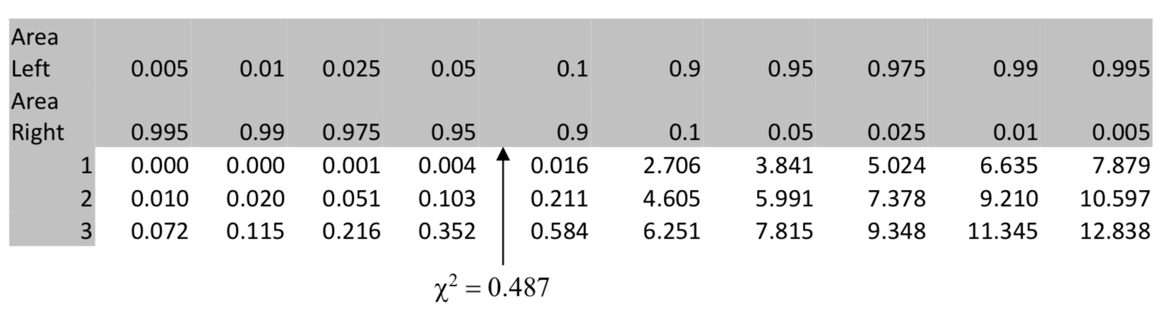
The table shows the p-value is less than 0.05. The calculator confirms this because \(\chi^2\) cdf (0.486, 1E99, 3) = 0.9218. Consequently the conclusion is that there is not a significant difference between the distribution of hurricanes in 1951-2000 and 1901-50.
Distinguishing between the use of the test of independence and homogeneity
While the mathematics behind both the test of independence and the test of homogeneity are the same, the intent behind their usage and interpretation of the results is different.
The test for independence is used when two random variables, both of which are considered to be response variables, are determined for each unit. The test for homogeneity is used when one of the random variables is the explanatory variable and subjects are selected based on their level of this variable. The other random variable is the response variable.
The determination of which test to used is established by the sampling approach. If two populations are clearly defined beforehand and a random selection is made from each population, then the populations will be compared using the test of homogeneity. If no effort is made to distinguish populations beforehand, and a random selection is made from this population and then the values of the two random variables are determined, the test of independence is appropriate.
An example may clarify the subtle difference between the two tests. Consider one random variable to be a person’s preference between running and swimming for exercise and the other random variable to be a person’s preference between watching TV or reading a book. If the researcher randomly selects some runners and some swimmers and asks each group about their preference for TV or reading a book, the test for homogeneity would be appropriate. On the other hand, if the researcher survey’s randomly selected people and asks if they prefer running or swimming and if they prefer TV or reading, then the objective will be to determine if there is a correlation between these two random variables by using the test of independence.
| Chi - Square Distributions | ||||||||||
| Area Left | 0.005 | 0.01 | 0.025 | 0.05 | 0.1 | 0.9 | 0.95 | 0.975 | 0.99 | 0.995 |
| Area Right | 0.995 | 0.99 | 0.975 | 0.95 | 0.9 | 0.1 | 0.05 | 0.025 | 0.01 | 0.005 |
| df | ||||||||||
| 1 | 0.000 | 0.000 | 0.001 | 0.004 | 0.016 | 2.706 | 3.841 | 5.024 | 6.635 | 7.879 |
| 2 | 0.010 | 0.020 | 0.051 | 0.103 | 0.211 | 4.605 | 5.991 | 7.378 | 9.210 | 10.597 |
| 3 | 0.072 | 0.115 | 0.216 | 0.352 | 0.584 | 6.251 | 7.815 | 9.348 | 11.345 | 12.838 |
| 4 | 0.207 | 0.287 | 0.484 | 0.711 | 1.064 | 7.779 | 9.488 | 11.143 | 13.277 | 14.860 |
| 5 | 0.412 | 0.554 | 0.831 | 1.145 | 1.610 | 9.236 | 11.070 | 12.832 | 15.086 | 16.750 |
| 6 | 0.676 | 0.872 | 1.237 | 1.635 | 2.204 | 10.645 | 12.592 | 14.449 | 16.812 | 18.548 |
| 7 | 0.989 | 1.239 | 1.690 | 2.167 | 2.833 | 12.017 | 14.067 | 16.013 | 18.475 | 20.278 |
| 8 | 1.344 | 1.647 | 2.180 | 2.733 | 3,490 | 13.362 | 15.507 | 17.535 | 20.090 | 21.955 |
| 9 | 1.735 | 2.088 | 2.700 | 3.325 | 4.168 | 14.684 | 16.919 | 19.023 | 21.666 | 23.589 |
| 10 | 2.156 | 2.558 | 3.247 | 3.940 | 4.865 | 15.987 | 18.307 | 20.483 | 23.209 | 25.188 |
| 11 | 2.603 | 3.053 | 3.816 | 4.575 | 5.578 | 17.275 | 19.675 | 21.920 | 24.725 | 26.757 |
| 12 | 3.074 | 3.571 | 4.404 | 5.226 | 6.304 | 18.549 | 21.026 | 23.337 | 26.217 | 28.300 |
| 13 | 3.565 | 4.107 | 5.009 | 5.892 | 7.041 | 19.812 | 22.362 | 24.736 | 27.688 | 29.819 |
| 14 | 4.075 | 4.660 | 5.629 | 6.571 | 7.790 | 21/064 | 23.685 | 26.119 | 29.141 | 31.319 |
| 15 | 4.601 | 5.229 | 6.262 | 7.261 | 8.547 | 22.307 | 24.996 | 27.488 | 30.578 | 32.801 |
| 16 | 5.142 | 5,812 | 6.908 | 7.962 | 9.312 | 23.542 | 26.296 | 28.845 | 32.000 | 34.267 |
| 17 | 5.697 | 6.408 | 7.564 | 8.672 | 10.085 | 24.769 | 27.587 | 30.191 | 33.409 | 35.718 |
| 18 | 6.265 | 7.015 | 8.231 | 9.390 | 10.865 | 25.989 | 28.869 | 31.526 | 34.805 | 37.156 |
| 19 | 6.844 | 7.633 | 8.907 | 10.117 | 11.651 | 27.204 | 30.144 | 32.852 | 36.191 | 38.582 |
| 20 | 7.434 | 8.260 | 9.591 | 10.851 | 12.443 | 28.412 | 31.410 | 34.170 | 37.566 | 39.997 |
| 21 | 8.034 | 8.897 | 10.283 | 11.591 | 13.240 | 29.615 | 32.671 | 35.479 | 38.932 | 41.401 |
| 22 | 8.643 | 9.542 | 10.982 | 12.338 | 14.041 | 30.813 | 33.924 | 36.781 | 40.289 | 42.796 |
| 23 | 9.260 | 10.196 | 11.689 | 13.091 | 14.848 | 32.007 | 35.172 | 38.076 | 41.638 | 44.181 |
| 24 | 9.886 | 10.856 | 12.401 | 13.848 | 15.659 | 33.196 | 36.415 | 39.365 | 42.980 | 45.558 |
| 25 | 10.520 | 11.524 | 13.120 | 14.611 | 16.473 | 34.382 | 37.652 | 40.646 | 44.314 | 46.928 |
| 26 | 11.160 | 12.198 | 13.844 | 15.379 | 17.292 | 35.563 | 38.885 | 41.923 | 45.642 | 48.290 |
| 27 | 11.808 | 12.878 | 14.573 | 16.151 | 18.114 | 36.741 | 40.113 | 43.195 | 46.963 | 49.645 |
| 28 | 12.461 | 13.565 | 15.398 | 16.928 | 18.939 | 37.916 | 41.337 | 44.461 | 48.278 | 50.994 |
| 29 | 13.121 | 14.256 | 16.047 | 17.708 | 19.768 | 39.087 | 42.557 | 45.722 | 49.588 | 52.335 |
| 30 | 13.787 | 14.953 | 16.791 | 18.493 | 20.599 | 40.256 | 43.773 | 46.979 | 50.892 | 53.672 |
| 40 | 20.707 | 22.164 | 24.433 | 26.509 | 29.051 | 51.805 | 55.758 | 59.342 | 63.691 | 66.766 |
| 50 | 27.991 | 29.707 | 32.357 | 34.764 | 37.689 | 63.167 | 67.505 | 71.420 | 76.154 | 79.490 |
| 60 | 35.534 | 37.485 | 40.482 | 43.188 | 46.459 | 74.397 | 79.082 | 83.298 | 88.379 | 91.952 |
| 70 | 43.275 | 45.442 | 48.758 | 51.739 | 55.329 | 85.527 | 90.531 | 95.023 | 100.425 | 104.215 |
| 80 | 51.172 | 53.540 | 57.153 | 60.391 | 64.278 | 96.578 | 101.879 | 106.629 | 112.329 | 116.321 |
| 90 | 59.196 | 61.754 | 65.647 | 69.126 | 73.291 | 107.565 | 113.145 | 118.136 | 124.116 | 128.299 |
| 100 | 67.328 | 70.065 | 74.222 | 77.929 | 82.358 | 118.498 | 124.342 | 129.561 | 135.807 | 140.170 |
| 110 | 75.550 | 78.458 | 82.867 | 86.792 | 91.471 | 129.385 | 135.480 | 140.916 | 147.414 | 151.948 |