7.E: Analysis of Bivariate Quantitative Data (Exercises)
- Page ID
- 5435
\( \newcommand{\vecs}[1]{\overset { \scriptstyle \rightharpoonup} {\mathbf{#1}} } \)
\( \newcommand{\vecd}[1]{\overset{-\!-\!\rightharpoonup}{\vphantom{a}\smash {#1}}} \)
\( \newcommand{\id}{\mathrm{id}}\) \( \newcommand{\Span}{\mathrm{span}}\)
( \newcommand{\kernel}{\mathrm{null}\,}\) \( \newcommand{\range}{\mathrm{range}\,}\)
\( \newcommand{\RealPart}{\mathrm{Re}}\) \( \newcommand{\ImaginaryPart}{\mathrm{Im}}\)
\( \newcommand{\Argument}{\mathrm{Arg}}\) \( \newcommand{\norm}[1]{\| #1 \|}\)
\( \newcommand{\inner}[2]{\langle #1, #2 \rangle}\)
\( \newcommand{\Span}{\mathrm{span}}\)
\( \newcommand{\id}{\mathrm{id}}\)
\( \newcommand{\Span}{\mathrm{span}}\)
\( \newcommand{\kernel}{\mathrm{null}\,}\)
\( \newcommand{\range}{\mathrm{range}\,}\)
\( \newcommand{\RealPart}{\mathrm{Re}}\)
\( \newcommand{\ImaginaryPart}{\mathrm{Im}}\)
\( \newcommand{\Argument}{\mathrm{Arg}}\)
\( \newcommand{\norm}[1]{\| #1 \|}\)
\( \newcommand{\inner}[2]{\langle #1, #2 \rangle}\)
\( \newcommand{\Span}{\mathrm{span}}\) \( \newcommand{\AA}{\unicode[.8,0]{x212B}}\)
\( \newcommand{\vectorA}[1]{\vec{#1}} % arrow\)
\( \newcommand{\vectorAt}[1]{\vec{\text{#1}}} % arrow\)
\( \newcommand{\vectorB}[1]{\overset { \scriptstyle \rightharpoonup} {\mathbf{#1}} } \)
\( \newcommand{\vectorC}[1]{\textbf{#1}} \)
\( \newcommand{\vectorD}[1]{\overrightarrow{#1}} \)
\( \newcommand{\vectorDt}[1]{\overrightarrow{\text{#1}}} \)
\( \newcommand{\vectE}[1]{\overset{-\!-\!\rightharpoonup}{\vphantom{a}\smash{\mathbf {#1}}}} \)
\( \newcommand{\vecs}[1]{\overset { \scriptstyle \rightharpoonup} {\mathbf{#1}} } \)
\( \newcommand{\vecd}[1]{\overset{-\!-\!\rightharpoonup}{\vphantom{a}\smash {#1}}} \)
\(\newcommand{\avec}{\mathbf a}\) \(\newcommand{\bvec}{\mathbf b}\) \(\newcommand{\cvec}{\mathbf c}\) \(\newcommand{\dvec}{\mathbf d}\) \(\newcommand{\dtil}{\widetilde{\mathbf d}}\) \(\newcommand{\evec}{\mathbf e}\) \(\newcommand{\fvec}{\mathbf f}\) \(\newcommand{\nvec}{\mathbf n}\) \(\newcommand{\pvec}{\mathbf p}\) \(\newcommand{\qvec}{\mathbf q}\) \(\newcommand{\svec}{\mathbf s}\) \(\newcommand{\tvec}{\mathbf t}\) \(\newcommand{\uvec}{\mathbf u}\) \(\newcommand{\vvec}{\mathbf v}\) \(\newcommand{\wvec}{\mathbf w}\) \(\newcommand{\xvec}{\mathbf x}\) \(\newcommand{\yvec}{\mathbf y}\) \(\newcommand{\zvec}{\mathbf z}\) \(\newcommand{\rvec}{\mathbf r}\) \(\newcommand{\mvec}{\mathbf m}\) \(\newcommand{\zerovec}{\mathbf 0}\) \(\newcommand{\onevec}{\mathbf 1}\) \(\newcommand{\real}{\mathbb R}\) \(\newcommand{\twovec}[2]{\left[\begin{array}{r}#1 \\ #2 \end{array}\right]}\) \(\newcommand{\ctwovec}[2]{\left[\begin{array}{c}#1 \\ #2 \end{array}\right]}\) \(\newcommand{\threevec}[3]{\left[\begin{array}{r}#1 \\ #2 \\ #3 \end{array}\right]}\) \(\newcommand{\cthreevec}[3]{\left[\begin{array}{c}#1 \\ #2 \\ #3 \end{array}\right]}\) \(\newcommand{\fourvec}[4]{\left[\begin{array}{r}#1 \\ #2 \\ #3 \\ #4 \end{array}\right]}\) \(\newcommand{\cfourvec}[4]{\left[\begin{array}{c}#1 \\ #2 \\ #3 \\ #4 \end{array}\right]}\) \(\newcommand{\fivevec}[5]{\left[\begin{array}{r}#1 \\ #2 \\ #3 \\ #4 \\ #5 \\ \end{array}\right]}\) \(\newcommand{\cfivevec}[5]{\left[\begin{array}{c}#1 \\ #2 \\ #3 \\ #4 \\ #5 \\ \end{array}\right]}\) \(\newcommand{\mattwo}[4]{\left[\begin{array}{rr}#1 \amp #2 \\ #3 \amp #4 \\ \end{array}\right]}\) \(\newcommand{\laspan}[1]{\text{Span}\{#1\}}\) \(\newcommand{\bcal}{\cal B}\) \(\newcommand{\ccal}{\cal C}\) \(\newcommand{\scal}{\cal S}\) \(\newcommand{\wcal}{\cal W}\) \(\newcommand{\ecal}{\cal E}\) \(\newcommand{\coords}[2]{\left\{#1\right\}_{#2}}\) \(\newcommand{\gray}[1]{\color{gray}{#1}}\) \(\newcommand{\lgray}[1]{\color{lightgray}{#1}}\) \(\newcommand{\rank}{\operatorname{rank}}\) \(\newcommand{\row}{\text{Row}}\) \(\newcommand{\col}{\text{Col}}\) \(\renewcommand{\row}{\text{Row}}\) \(\newcommand{\nul}{\text{Nul}}\) \(\newcommand{\var}{\text{Var}}\) \(\newcommand{\corr}{\text{corr}}\) \(\newcommand{\len}[1]{\left|#1\right|}\) \(\newcommand{\bbar}{\overline{\bvec}}\) \(\newcommand{\bhat}{\widehat{\bvec}}\) \(\newcommand{\bperp}{\bvec^\perp}\) \(\newcommand{\xhat}{\widehat{\xvec}}\) \(\newcommand{\vhat}{\widehat{\vvec}}\) \(\newcommand{\uhat}{\widehat{\uvec}}\) \(\newcommand{\what}{\widehat{\wvec}}\) \(\newcommand{\Sighat}{\widehat{\Sigma}}\) \(\newcommand{\lt}{<}\) \(\newcommand{\gt}{>}\) \(\newcommand{\amp}{&}\) \(\definecolor{fillinmathshade}{gray}{0.9}\)Chapter 7 Homework
In the first problem, all calculations, except finding the correlation, should be done using the formulas and tables. For the remaining problems you may use either the calculator or Excel.
- In the game of baseball the objective is to win games by scoring more runs than the opposing team. Runs can only be scored if someone gets on base. Traditionally, batting average (which is actually a proportion of hits to at bats) has been used as one of the primary measures of player success. An alternative is slugging percent which is the ratio of total number of bases reached during an at bat to the number of at bats. A walk or single counts as one base, a double counts as two bases, etc. The table below contains the batting average, slugging percentage, and runs scored from 10 Major League Baseball teams randomly selected from the 2012 and 2013 seasons.(http://www.fangraphs.com, 12-12-13)
Team Batting Average Team Slugging Percentage Team Runs Scored 0.242 0.380 614 0.231 0.335 513 0.283 0.434 796 0.240 0.375 610 0.252 0.398 640 0.268 0.422 726 0.245 0.407 716 0.260 0.390 701 0.240 0.394 697 0.255 0.422 748 a. Make a scatter plot of team batting average and team runs scored. Label the graph completely.

b. Use your calculator to find the mean and standard deviation for batting average and runs scored. The correlation between these is 0.805.
Mean batting average _________ Standard deviation for batting average ___________
Mean runs scored ______________ Standard deviation for runs scored____________c. Use the appropriate t test statistic to determine if the correlation is significant at the 0.05 level of significance. Show the formula, substitution and the results in a complete concluding sentence.
Formula Substitution
Concluding sentence:
d. Find the equation of the regression line.
\(b = r(\dfrac{s_y}{s_x})\)
\(\bar{y} = a + b\bar{x}\)
Regression equation:
Draw this line on your scatter plot. (Hint: pick two different x values, one near either side of the x-axis, substitute into the regression equation to find y. Then plot the two (x, y) ordered pairs that you produced. This is how you learned to graph in Algebra using a table of values).
e. What is the \(r^2\) value and what does it mean?
f. Predict the number of runs scored for a team with a batting average of 0.250.
g. Repeat this entire problem for slugging percent and runs scored, only this time use the LinRegTTest function on your calculator.

Correlation _____________
Hypothesis test concluding sentence
Regression equation _________________________
Coefficient of determination (\(R^2\)) ____________
Predict the number of runs scored for a team with a slugging percentage of 0.400. __________________
Compare and contrast the results from the analysis of batting average and slugging percentage and their relationship to runs scored.
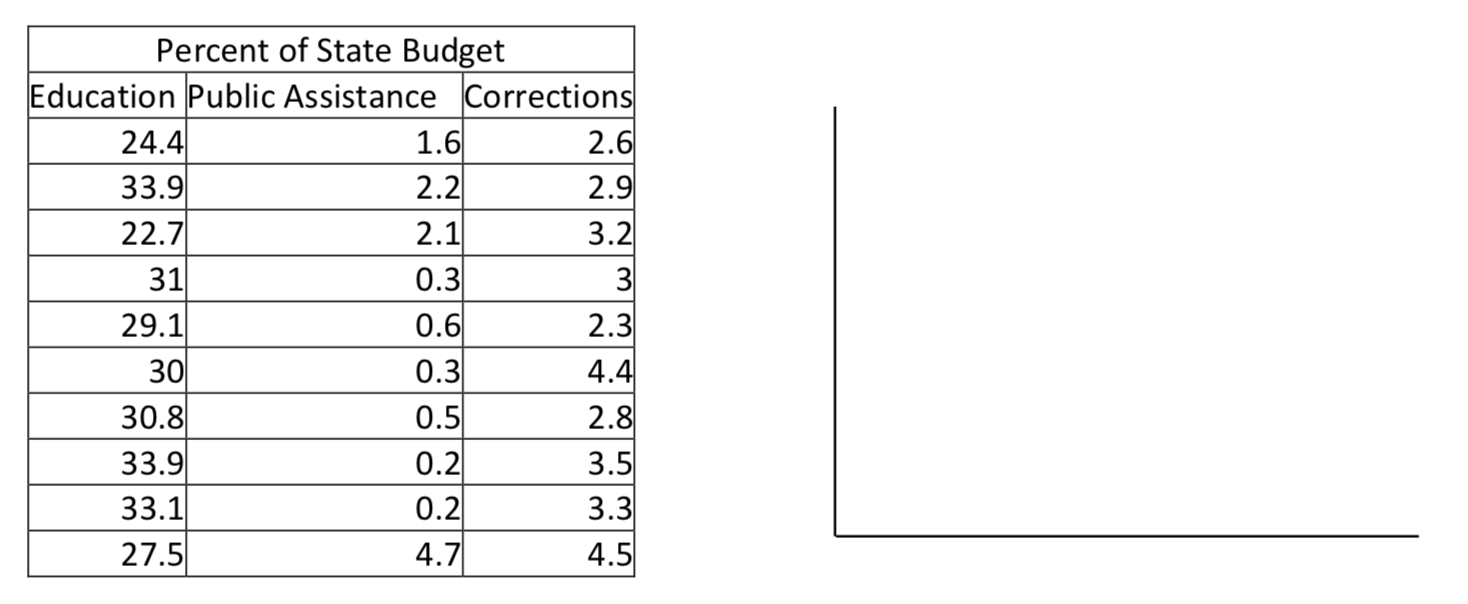
- In an ideal society, crime would seldom happen and consequently the population’s financial resources could be spent on other things that benefit society. The primary categories for state spending are k-12 education, higher education, public assistance, Medicaid, transportation and corrections. Many of us in the field of education believe that it is critical for the country and holds the possibility of reducing both crime and public assistance. Is there a significant correlation between the percent of state budgets spent on k-12 and higher education and the percent spent on public assistance? Is there a significant correlation between the percent of state budgets spent on education and corrections? Data is from 2011.(www.nasbo.org/sites/default/f...20Report_1.pdf 12-12-13.)

a. Make a scatter plot, use your calculator to test the hypothesis that there is a correlation between education spending and public assistance spending. Show calculator outputs including the correlation, \(r^2\) value and equation of the regression line. Write a statistical conclusion then interpret the results. Use a level of significance of 0.05.
Correlation ____________
Coefficient of determination (\(r^2\) value) _______________Regression equation _____________________
What does \(x\) represent in this equation? ______________
What does \(y\) represent in this equation? ______________Hypothesis test concluding sentence:
b. Make a scatter plot, use your calculator to test the hypothesis that there is a correlation between education spending and corrections spending. Show calculator outputs including the correlation, \(r^2\) value and equation of the regression line. Write a statistical conclusion then interpret the results. Use a level of significance of 0.05.

Correlation ____________
Coefficient of determination (\(r^2\) value) _______________Regression equation _____________________
What does \(x\) represent in this equation? ______________
What does \(y\) represent in this equation? ______________Hypothesis test concluding sentence:
- Is there a correlation between the population of a state and the median income in the state? (Data from http://www.city-data.com/ 12-12-13.)
State Population (millions) Median income ($) 2.7 55764 2.8 49444 2 43569 7.9 61090 9.6 48448 1.3 46405 11.5 46563 2.7 54065 4.5 43362 Make a scatter plot, use your calculator to test the hypothesis that there is a correlation between population and median income. Show calculator outputs including the correlation, r2 value and equation of the regression line. Write a statistical conclusion then interpret the results. Use a level of significance of 0.05.

Correlation ____________
Coefficient of determination (\(r^2\) value) _______________Regression equation _____________________
What does \(x\) represent in this equation? ______________
What does \(y\) represent in this equation? ______________Hypothesis test concluding sentence:
- One theory about the benefit of large cities is that they serve as a hub for creativity due to the frequent interactions between people. One measure of creative problem solving is the number of patents that are granted. Is there a correlation between the size of a metropolitan or micropolitan area and the number of patents that were granted to someone in that area?(www.uspto.gov/web/offices/ac/...allcbsa_gd.htm andwww.census.gov/popfinder/ (12-12-13))

a. Make a scatter plot, use your calculator to test the hypothesis that there is a correlation between population and total patents 2000-2011. Show calculator outputs including the correlation, \(r^2\) value and equation of the regression line. Write a statistical conclusion then interpret the results. Use a level of significance of 0.05.Correlation ____________
Coefficient of determination (\(r^2\) value) _______________Regression equation _____________________
What does \(x\) represent in this equation? ______________
What does \(y\) represent in this equation? ______________Hypothesis test concluding sentence:
b. There are two outliers in this data. Do you think they have too great an influence on the correlation and therefore should be removed or do you think they are relevant and should be kept with the data?
c. Use the regression line to predict the number of patents for a city with 60,000 people. - Why Statistical Reasoning is Important for Anatomy and Physiology Students and Professionals In collaboration with Barry Putman, Professor of Biology, Natural Science Coordinator, JBLM
This topic is discussed in the following Pierce College Course: Biol 241
briefing 8.1
Near Point of Accommodation (NPA) is the nearest point at which the eyes can comfortably focus. In the lab conducted in the anatomy and physiology class, students will hold a meter stick against their forehead, close their left eye and with their right eye they will focus on a small ruler held against the meter stick. With the ruler starting at arm’s length they will slowly move it toward their eye. When they reach the point where the ruler has the greatest focus (NPA), a partner will record the distance, in centimeters, from their eye.
Since people often need glasses later in life, it would be reasonable to determine if there is a correlation between a person’s age and their NPA. Consequently, students in the study record both their age and NPA.
a. Of the two variables, NPA and age, which should be the explanatory variable? Why?
b. Of the two variables, NPA and age, which should be the response variable? Why?
c. There were 103 data values made available for this problem. This number will be reduced using a random process to save you time. If a systematic sampling method is used with every \(10^{\text{th}}\) value selected, what are the 10 or 11 numbers that would be selected if the calculator is seeded with a 31?
, , , , , , , , , ,
The table below contains the data.Age 26 28 30 26 36 19 20 20 27 25 24 NPA 31 13 36 22 34 8 8 10 24 14 11 d. Make a scatter plot. Write a complete sentence explaining your interpretation of the graph.
e. Use your calculator to find the sample correlation.
f. Write and test the hypotheses to determine if there is a significant correlation in the population. Use a 0.05 level of significance. Write a concluding sentence.
g. What type error could have been made?
h. What do you conclude about the relationship between age and NPA?


