27.1: Linear Regression (Section 26.1)

Last updated
Save as PDF

Page ID: 8858

\( \newcommand{\vecs}[1]{\overset { \scriptstyle \rightharpoonup} {\mathbf{#1}} } \) \( \newcommand{\vecd}[1]{\overset{-\!-\!\rightharpoonup}{\vphantom{a}\smash {#1}}} \)\(\newcommand{\id}{\mathrm{id}}\) \( \newcommand{\Span}{\mathrm{span}}\) \( \newcommand{\kernel}{\mathrm{null}\,}\) \( \newcommand{\range}{\mathrm{range}\,}\) \( \newcommand{\RealPart}{\mathrm{Re}}\) \( \newcommand{\ImaginaryPart}{\mathrm{Im}}\) \( \newcommand{\Argument}{\mathrm{Arg}}\) \( \newcommand{\norm}[1]{\| #1 \|}\) \( \newcommand{\inner}[2]{\langle #1, #2 \rangle}\) \( \newcommand{\Span}{\mathrm{span}}\) \(\newcommand{\id}{\mathrm{id}}\) \( \newcommand{\Span}{\mathrm{span}}\) \( \newcommand{\kernel}{\mathrm{null}\,}\) \( \newcommand{\range}{\mathrm{range}\,}\) \( \newcommand{\RealPart}{\mathrm{Re}}\) \( \newcommand{\ImaginaryPart}{\mathrm{Im}}\) \( \newcommand{\Argument}{\mathrm{Arg}}\) \( \newcommand{\norm}[1]{\| #1 \|}\) \( \newcommand{\inner}[2]{\langle #1, #2 \rangle}\) \( \newcommand{\Span}{\mathrm{span}}\)\(\newcommand{\AA}{\unicode[.8,0]{x212B}}\)

To perform linear regression in R, we use the lm() function. Let’s generate some data and use this function to compute the linear regression solution.

npoints <- 100
intercept = 10
# slope of X/Y relationship
slope=0.5
# this lets us control the strength of the relationship
# by varying the amount of noise added to the y variable
noise_sd = 0.6

regression_data <- tibble(x = rnorm(npoints)) %>%
  mutate(y = x*slope + rnorm(npoints)*noise_sd + intercept)

ggplot(regression_data,aes(x,y)) + 
  geom_point()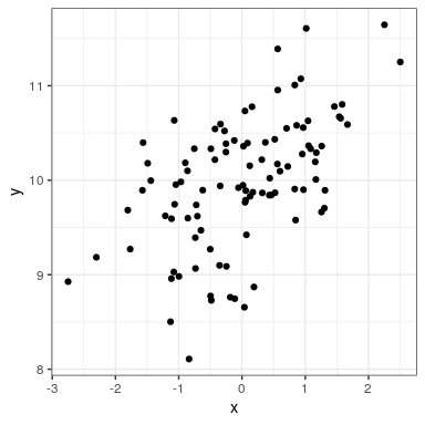

We can then apply lm() to these data:

lm_result <- lm(y ~ x, data=regression_data)
summary(lm_result)

## 
## Call:
## lm(formula = y ~ x, data = regression_data)
## 
## Residuals:
##     Min      1Q  Median      3Q     Max 
## -1.5563 -0.3042 -0.0059  0.3804  1.2522 
## 
## Coefficients:
##             Estimate Std. Error t value Pr(>|t|)    
## (Intercept)   9.9761     0.0580  172.12  < 2e-16 ***
## x             0.3725     0.0586    6.35  6.6e-09 ***
## ---
## Signif. codes:  0 '***' 0.001 '**' 0.01 '*' 0.05 '.' 0.1 ' ' 1
## 
## Residual standard error: 0.58 on 98 degrees of freedom
## Multiple R-squared:  0.292,  Adjusted R-squared:  0.284 
## F-statistic: 40.4 on 1 and 98 DF,  p-value: 6.65e-09

We should see three things in the lm() results:

The estimate of the Intercept in the model should be very close to the intercept that we specified
The estimate for the x parameter should be very close to the slope that we specified
The residual standard error should be roughly similar to the noise standard deviation that we specified