7.3: Population Model
- Page ID
- 2913
\( \newcommand{\vecs}[1]{\overset { \scriptstyle \rightharpoonup} {\mathbf{#1}} } \)
\( \newcommand{\vecd}[1]{\overset{-\!-\!\rightharpoonup}{\vphantom{a}\smash {#1}}} \)
\( \newcommand{\id}{\mathrm{id}}\) \( \newcommand{\Span}{\mathrm{span}}\)
( \newcommand{\kernel}{\mathrm{null}\,}\) \( \newcommand{\range}{\mathrm{range}\,}\)
\( \newcommand{\RealPart}{\mathrm{Re}}\) \( \newcommand{\ImaginaryPart}{\mathrm{Im}}\)
\( \newcommand{\Argument}{\mathrm{Arg}}\) \( \newcommand{\norm}[1]{\| #1 \|}\)
\( \newcommand{\inner}[2]{\langle #1, #2 \rangle}\)
\( \newcommand{\Span}{\mathrm{span}}\)
\( \newcommand{\id}{\mathrm{id}}\)
\( \newcommand{\Span}{\mathrm{span}}\)
\( \newcommand{\kernel}{\mathrm{null}\,}\)
\( \newcommand{\range}{\mathrm{range}\,}\)
\( \newcommand{\RealPart}{\mathrm{Re}}\)
\( \newcommand{\ImaginaryPart}{\mathrm{Im}}\)
\( \newcommand{\Argument}{\mathrm{Arg}}\)
\( \newcommand{\norm}[1]{\| #1 \|}\)
\( \newcommand{\inner}[2]{\langle #1, #2 \rangle}\)
\( \newcommand{\Span}{\mathrm{span}}\) \( \newcommand{\AA}{\unicode[.8,0]{x212B}}\)
\( \newcommand{\vectorA}[1]{\vec{#1}} % arrow\)
\( \newcommand{\vectorAt}[1]{\vec{\text{#1}}} % arrow\)
\( \newcommand{\vectorB}[1]{\overset { \scriptstyle \rightharpoonup} {\mathbf{#1}} } \)
\( \newcommand{\vectorC}[1]{\textbf{#1}} \)
\( \newcommand{\vectorD}[1]{\overrightarrow{#1}} \)
\( \newcommand{\vectorDt}[1]{\overrightarrow{\text{#1}}} \)
\( \newcommand{\vectE}[1]{\overset{-\!-\!\rightharpoonup}{\vphantom{a}\smash{\mathbf {#1}}}} \)
\( \newcommand{\vecs}[1]{\overset { \scriptstyle \rightharpoonup} {\mathbf{#1}} } \)
\( \newcommand{\vecd}[1]{\overset{-\!-\!\rightharpoonup}{\vphantom{a}\smash {#1}}} \)
\(\newcommand{\avec}{\mathbf a}\) \(\newcommand{\bvec}{\mathbf b}\) \(\newcommand{\cvec}{\mathbf c}\) \(\newcommand{\dvec}{\mathbf d}\) \(\newcommand{\dtil}{\widetilde{\mathbf d}}\) \(\newcommand{\evec}{\mathbf e}\) \(\newcommand{\fvec}{\mathbf f}\) \(\newcommand{\nvec}{\mathbf n}\) \(\newcommand{\pvec}{\mathbf p}\) \(\newcommand{\qvec}{\mathbf q}\) \(\newcommand{\svec}{\mathbf s}\) \(\newcommand{\tvec}{\mathbf t}\) \(\newcommand{\uvec}{\mathbf u}\) \(\newcommand{\vvec}{\mathbf v}\) \(\newcommand{\wvec}{\mathbf w}\) \(\newcommand{\xvec}{\mathbf x}\) \(\newcommand{\yvec}{\mathbf y}\) \(\newcommand{\zvec}{\mathbf z}\) \(\newcommand{\rvec}{\mathbf r}\) \(\newcommand{\mvec}{\mathbf m}\) \(\newcommand{\zerovec}{\mathbf 0}\) \(\newcommand{\onevec}{\mathbf 1}\) \(\newcommand{\real}{\mathbb R}\) \(\newcommand{\twovec}[2]{\left[\begin{array}{r}#1 \\ #2 \end{array}\right]}\) \(\newcommand{\ctwovec}[2]{\left[\begin{array}{c}#1 \\ #2 \end{array}\right]}\) \(\newcommand{\threevec}[3]{\left[\begin{array}{r}#1 \\ #2 \\ #3 \end{array}\right]}\) \(\newcommand{\cthreevec}[3]{\left[\begin{array}{c}#1 \\ #2 \\ #3 \end{array}\right]}\) \(\newcommand{\fourvec}[4]{\left[\begin{array}{r}#1 \\ #2 \\ #3 \\ #4 \end{array}\right]}\) \(\newcommand{\cfourvec}[4]{\left[\begin{array}{c}#1 \\ #2 \\ #3 \\ #4 \end{array}\right]}\) \(\newcommand{\fivevec}[5]{\left[\begin{array}{r}#1 \\ #2 \\ #3 \\ #4 \\ #5 \\ \end{array}\right]}\) \(\newcommand{\cfivevec}[5]{\left[\begin{array}{c}#1 \\ #2 \\ #3 \\ #4 \\ #5 \\ \end{array}\right]}\) \(\newcommand{\mattwo}[4]{\left[\begin{array}{rr}#1 \amp #2 \\ #3 \amp #4 \\ \end{array}\right]}\) \(\newcommand{\laspan}[1]{\text{Span}\{#1\}}\) \(\newcommand{\bcal}{\cal B}\) \(\newcommand{\ccal}{\cal C}\) \(\newcommand{\scal}{\cal S}\) \(\newcommand{\wcal}{\cal W}\) \(\newcommand{\ecal}{\cal E}\) \(\newcommand{\coords}[2]{\left\{#1\right\}_{#2}}\) \(\newcommand{\gray}[1]{\color{gray}{#1}}\) \(\newcommand{\lgray}[1]{\color{lightgray}{#1}}\) \(\newcommand{\rank}{\operatorname{rank}}\) \(\newcommand{\row}{\text{Row}}\) \(\newcommand{\col}{\text{Col}}\) \(\renewcommand{\row}{\text{Row}}\) \(\newcommand{\nul}{\text{Nul}}\) \(\newcommand{\var}{\text{Var}}\) \(\newcommand{\corr}{\text{corr}}\) \(\newcommand{\len}[1]{\left|#1\right|}\) \(\newcommand{\bbar}{\overline{\bvec}}\) \(\newcommand{\bhat}{\widehat{\bvec}}\) \(\newcommand{\bperp}{\bvec^\perp}\) \(\newcommand{\xhat}{\widehat{\xvec}}\) \(\newcommand{\vhat}{\widehat{\vvec}}\) \(\newcommand{\uhat}{\widehat{\uvec}}\) \(\newcommand{\what}{\widehat{\wvec}}\) \(\newcommand{\Sighat}{\widehat{\Sigma}}\) \(\newcommand{\lt}{<}\) \(\newcommand{\gt}{>}\) \(\newcommand{\amp}{&}\) \(\definecolor{fillinmathshade}{gray}{0.9}\)Our regression model is based on a sample of n bivariate observations drawn from a larger population of measurements.
\[\hat y = b_0 +b_1x\]
We use the means and standard deviations of our sample data to compute the slope (b1) and y-intercept (b0) in order to create an ordinary least-squares regression line. But we want to describe the relationship between y and x in the population, not just within our sample data. We want to construct a population model. Now we will think of the least-squares line computed from a sample as an estimate of the true regression line for the population.
\(\mu_y = \beta_0 + \beta_1x\), where \(\mu_y\) is the population mean response, \(\beta_0\) is the y-intercept, and \(beta_1\) is the slope for the population model.
In our population, there could be many different responses for a value of x. In simple linear regression, the model assumes that for each value of x the observed values of the response variable y are normally distributed with a mean that depends on x. We use μy to represent these means. We also assume that these means all lie on a straight line when plotted against x (a line of means).
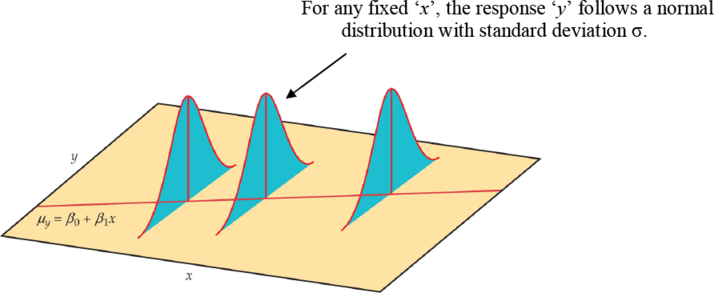
Figure \(\PageIndex{1}\). . The statistical model for linear regression; the mean response is a straight-line function of the predictor variable.
The sample data then fit the statistical model:
Data = fit + residual
\[y_i = (\beta_0 + \beta_1x_i)+\epsilon_i\]
where the errors (εi) are independent and normally distributed N (0, σ). Linear regression also assumes equal variance of y (σ is the same for all values of x). We use ε (Greek epsilon) to stand for the residual part of the statistical model. A response y is the sum of its mean and chance deviation εfrom the mean. The deviations ε represents the “noise” in the data. In other words, the noise is the variation in y due to other causes that prevent the observed (x, y) from forming a perfectly straight line.
The sample data used for regression are the observed values of y and x. The response y to a given xis a random variable, and the regression model describes the mean and standard deviation of this random variable y. The intercept β0, slope β1, and standard deviation σ of y are the unknown parameters of the regression model and must be estimated from the sample data.
- The value of ŷ from the least squares regression line is really a prediction of the mean value of y (μy) for a given value of x.
- The least squares regression line (\(\hat y = b_0+b_1x\)) obtained from sample data is the best estimate of the true population regression line
(\(\mu_y = \beta_0 + \beta_1x\)).
ŷ is an unbiased estimate for the mean response μy
b0 is an unbiased estimate for the intercept β0
b1 is an unbiased estimate for the slope β1
Parameter Estimation
Once we have estimates of β0 and β1 (from our sample data b0 and b1), the linear relationship determines the estimates of μy for all values of x in our population, not just for the observed values of x. We now want to use the least-squares line as a basis for inference about a population from which our sample was drawn.
Model assumptions tell us that b0 and b1 are normally distributed with means β0 and β1 with standard deviations that can be estimated from the data. Procedures for inference about the population regression line will be similar to those described in the previous chapter for means. As always, it is important to examine the data for outliers and influential observations.
In order to do this, we need to estimate σ, the regression standard error. This is the standard deviation of the model errors. It measures the variation of y about the population regression line. We will use the residuals to compute this value. Remember, the predicted value of y (p̂) for a specific x is the point on the regression line. It is the unbiased estimate of the mean response (μy) for that x. The residual is:
residual = observed – predicted
\[\epsilon_i = y_i – \hat {y} = y_i -(b_0+b_1x)\]
The residual ei corresponds to model deviation \(\epsilon_i\) where \(\sum \epsilon_i = 0\) with a mean of 0. The regression standard error s is an unbiased estimate of σ.
\[s=\sqrt {\dfrac {\sum residual^2}{n-2}} = \sqrt {\dfrac {\sum (y_i-\hat {y_i})^2}{n-2}}\]
The quantity s is the estimate of the regression standard error (σ) and \(s^2\) is often called the mean square error (MSE). A small value of s suggests that observed values of y fall close to the true regression line and the line \(\hat y = b_0 +b_1x\)should provide accurate estimates and predictions.
Confidence Intervals and Significance Tests for Model Parameters
In an earlier chapter, we constructed confidence intervals and did significance tests for the population parameter μ (the population mean). We relied on sample statistics such as the mean and standard deviation for point estimates, margins of errors, and test statistics. Inference for the population parameters β0 (slope) and β1 (y-intercept) is very similar.
Inference for the slope and intercept are based on the normal distribution using the estimates b0 and b1. The standard deviations of these estimates are multiples of σ, the population regression standard error. Remember, we estimate σ with s (the variability of the data about the regression line). Because we use s, we rely on the student t-distribution with (n – 2) degrees of freedom.
\[\sigma_{\hat{\beta_0}} = \sigma \sqrt { \frac {1}{n} + \dfrac {\bar x ^2}{\sum (x_i - \bar x)^2}}\]
The standard error for estimate of \(\beta_0\)
\[\sigma_{\hat{\beta_1}} = \sigma \sqrt { \frac {1}{n} + \dfrac {\bar x ^2}{\sum (x_i - \bar x)^2}}\]
The standard error for estimate of \(\beta_1\)
We can construct confidence intervals for the regression slope and intercept in much the same way as we did when estimating the population mean.
A confidence interval for \(\beta_0 : b_0 \pm t_{\alpha/2} SE_{b_0}\)
A confidence interval for \(\beta_1 : b_1 \pm t_{\alpha/2} SE_{b_1}\)
where \(SE_{b_0}\) and \(SE_{b_1}\) are the standard errors for the y-intercept and slope, respectively.
We can also test the hypothesis \(H_0: \beta_1 = 0\). When we substitute \(\beta_1 = 0\) in the model, the x-term drops out and we are left with \(\mu_y = \beta_0\). This tells us that the mean of y does NOT vary with x. In other words, there is no straight line relationship between x and y and the regression of y on x is of no value for predicting y.
Hypothesis test for \(\beta_1\)
\(H_0: \beta_1 =0\)
\(H_1: \beta_1 \ne 0\)
The test statistic is \(t = b_1 / SE_{b_1}\)
We can also use the F-statistic (MSR/MSE) in the regression ANOVA table*
*Recall that t2 = F
So let’s pull all of this together in an example.
The index of biotic integrity (IBI) is a measure of water quality in streams. As a manager for the natural resources in this region, you must monitor, track, and predict changes in water quality. You want to create a simple linear regression model that will allow you to predict changes in IBI in forested area. The following table conveys sample data from a coastal forest region and gives the data for IBI and forested area in square kilometers. Let forest area be the predictor variable (x) and IBI be the response variable (y).
\[ \begin{array}{ccccccccc}
\text { IBI } & \text { Forest Area } & \text { IBI } & \text { Forest Area } & \text { IBI } & \text { Forest Area } & \text { IBI } & \text { Forest Area } & \text { IBI } \\
47 & 38 & 41 & 22 & 61 & 43 & 71 & 79 & 84 \\
72 & 9 & 33 & 25 & 62 & 47 & 33 & 79 & 83 \\
21 & 10 & 23 & 31 & 18 & 49 & 59 & 80 & 82 \\
19 & 10 & 32 & 32 & 44 & 49 & 81 & 86 & 82 \\
72 & 52 & 80 & 33 & 30 & 52 & 71 & 89 & 86 \\
56 & 14 & 31 & 33 & 65 & 52 & 75 & 90 & 79 \\
49 & 66 & 78 & 33 & 78 & 59 & 64 & 95 & 67 \\
89 & 17 & 21 & 39 & 71 & 63 & 41 & 95 & 56 \\
43 & 18 & 43 & 41 & 60 & 68 & 82 & 100 & 85 \\
66 & 21 & 45 & 43 & 58 & 75 & 60 & 100 & 91
\end{array} \nonumber \]
Table \(\PageIndex{1}\). Observed data of biotic integrity and forest area.
Solution
We begin with a computing descriptive statistics and a scatterplot of IBI against Forest Area.
x̄ = 47.42; sx 27.37; ȳ = 58.80; sy = 21.38; r = 0.735
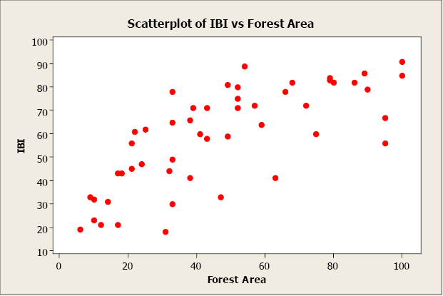
Figure \(\PageIndex{2}\). . Scatterplot of IBI vs. Forest Area.
There appears to be a positive linear relationship between the two variables. The linear correlation coefficient is r = 0.735. This indicates a strong, positive, linear relationship. In other words, forest area is a good predictor of IBI. Now let’s create a simple linear regression model using forest area to predict IBI (response).
First, we will compute b0 and b1 using the shortcut equations.
\[b_1 = r (\frac {s_y}{s_x}) = 0.735(\frac {21.38}{27.37})=0.574 \nonumber \]
\[b_0 =\bar y -b_1 \bar x =58.80-0.574 \times 47.42=31.581 \nonumber \]
The regression equation is
\[\hat y =31.58 + 0.574x \nonumber \]
Now let’s use Minitab to compute the regression model. The output appears below.
Regression Analysis: IBI versus Forest Area
The regression equation is IBI = 31.6 + 0.574 Forest Area
|
Predictor |
Coef |
SE Coef |
T |
P |
|
Constant |
31.583 |
4.177 |
7.56 |
0.000 |
|
Forest Area |
0.57396 |
0.07648 |
7.50 |
0.000 |
|
S = 14.6505 |
R-Sq = 54.0% |
R-Sq(adj) = 53.0% |
||
|
Analysis of Variance |
|||||
|
Source |
DF |
SS |
MS |
F |
P |
|
Regression |
1 |
12089 |
12089 |
56.32 |
0.000 |
|
Residual Error |
48 |
10303 |
215 |
||
|
Total |
49 |
22392 |
|||
The estimates for β0 and β1 are 31.6 and 0.574, respectively. We can interpret the y-intercept to mean that when there is zero forested area, the IBI will equal 31.6. For each additional square kilometer of forested area added, the IBI will increase by 0.574 units.
The coefficient of determination, R2, is 54.0%. This means that 54% of the variation in IBI is explained by this model. Approximately 46% of the variation in IBI is due to other factors or random variation. We would like R2 to be as high as possible (maximum value of 100%).
The residual and normal probability plots do not indicate any problems.

Figure \(\PageIndex{3}\). . A residual and normal probability plot.
The estimate of σ, the regression standard error, is s = 14.6505. This is a measure of the variation of the observed values about the population regression line. We would like this value to be as small as possible. The MSE is equal to 215. Remember, the \(\sqrt {MSE}=s\). The standard errors for the coefficients are 4.177 for the y-intercept and 0.07648 for the slope.
We know that the values b0 = 31.6 and b1 = 0.574 are sample estimates of the true, but unknown, population parameters β0 and β1. We can construct 95% confidence intervals to better estimate these parameters. The critical value (tα/2) comes from the student t-distribution with (n – 2) degrees of freedom. Our sample size is 50 so we would have 48 degrees of freedom. The closest table value is 2.009.
95% confidence intervals for β0 and β1
\[b_0 \pm t_{\alpha/2} SE_{b_0} = 31.6 \pm 2.009(4.177) = (23.21, 39.99) \nonumber \]
\[b_1 \pm t_{\alpha/2} SE_{b_1} = 0.574 \pm 2.009(0.07648) = (0.4204, 0.7277) \nonumber \]
The next step is to test that the slope is significantly different from zero using a 5% level of significance.
|
H0: β1 =0 |
H1: β1 ≠0 |
\[t = \frac {b_1} {SE_{b_1}} = \frac {0.574}{0.07648} = 7.50523 \nonumber \]
We have 48 degrees of freedom and the closest critical value from the student t-distribution is 2.009. The test statistic is greater than the critical value, so we will reject the null hypothesis. The slope is significantly different from zero. We have found a statistically significant relationship between Forest Area and IBI.
The Minitab output also report the test statistic and p-value for this test.
|
The regression equation is IBI = 31.6 + 0.574 Forest Area |
||||
|
Predictor |
Coef |
SE Coef |
T |
P |
|
Constant |
31.583 |
4.177 |
7.56 |
0.000 |
|
Forest Area |
0.57396 |
0.07648 |
7.50 |
0.000 |
|
S = 14.6505 |
R-Sq = 54.0% |
R-Sq(adj) = 53.0% |
||
|
Analysis of Variance |
|||||
|
Source |
DF |
SS |
MS |
F |
P |
|
Regression |
1 |
12089 |
12089 |
56.32 |
0.000 |
|
Residual Error |
48 |
10303 |
215 |
||
|
Total |
49 |
22392 |
|||
The t test statistic is 7.50 with an associated p-value of 0.000. The p-value is less than the level of significance (5%) so we will reject the null hypothesis. The slope is significantly different from zero. The same result can be found from the F-test statistic of 56.32 (7.5052 = 56.32). The p-value is the same (0.000) as the conclusion.
Confidence Interval for \(\mu_y\)
Now that we have created a regression model built on a significant relationship between the predictor variable and the response variable, we are ready to use the model for
- estimating the average value of y for a given value of x
- predicting a particular value of y for a given value of x
Let’s examine the first option. The sample data of n pairs that was drawn from a population was used to compute the regression coefficients b0 and b1 for our model, and gives us the average value of y for a specific value of x through our population model \(\mu_y = \beta_0 + \beta_1x\)
. For every specific value of x, there is an average y (μy), which falls on the straight line equation (a line of means). Remember, that there can be many different observed values of the y for a particular x, and these values are assumed to have a normal distribution with a mean equal to \(\beta_0 + \beta_1x\) and a variance of σ2. Since the computed values of b0 and b1 vary from sample to sample, each new sample may produce a slightly different regression equation. Each new model can be used to estimate a value of y for a value of x. How far will our estimator \(\hat y =b_0+b_1x\) be from the true population mean for that value of x? This depends, as always, on the variability in our estimator, measured by the standard error.
It can be shown that the estimated value of y when x = x0 (some specified value of x), is an unbiased estimator of the population mean, and that p̂ is normally distributed with a standard error of
\[\]SE_{\hat \mu} = s\sqrt {\frac {1}{n} + \frac {(x_0-\bar x)^2}{\sum (x_i - \bar x)^2}}\]
We can construct a confidence interval to better estimate this parameter (μy) following the same procedure illustrated previously in this chapter.
\[\]\hat {\mu_y} \pm t_{\alpha/2}SE_{\hat \mu}\]
where the critical value tα/2 comes from the student t-table with (n – 2) degrees of freedom.
Statistical software, such as Minitab, will compute the confidence intervals for you. Using the data from the previous example, we will use Minitab to compute the 95% confidence interval for the mean response for an average forested area of 32 km.
|
Predicted Values for New Observations |
|||
|
New Obs Fit |
SE Fit |
95% |
CI |
|
1 |
49.9496 |
2.38400 |
(45.1562,54.7429) |
If you sampled many areas that averaged 32 km. of forested area, your estimate of the average IBI would be from 45.1562 to 54.7429.
You can repeat this process many times for several different values of x and plot the confidence intervals for the mean response.
|
x |
95% CI |
|
20 |
(37.13, 48.88) |
|
40 |
(50.22, 58.86) |
|
60 |
(61.43, 70.61) |
|
80 |
(70.98, 84.02) |
|
100 |
(79.88, 98.07) |
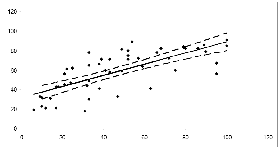
Figure \(\PageIndex{4}\). . 95% confidence intervals for the mean response.
Notice how the width of the 95% confidence interval varies for the different values of x. Since the confidence interval width is narrower for the central values of x, it follows that μy is estimated more precisely for values of x in this area. As you move towards the extreme limits of the data, the width of the intervals increases, indicating that it would be unwise to extrapolate beyond the limits of the data used to create this model.
Prediction Intervals
What if you want to predict a particular value of y when \(x = x_0\)? Or, perhaps you want to predict the next measurement for a given value of x? This problem differs from constructing a confidence interval for \(\mu_y\). Instead of constructing a confidence interval to estimate a population parameter, we need to construct a prediction interval. Choosing to predict a particular value of y incurs some additional error in the prediction because of the deviation of y from the line of means. Examine the figure below. You can see that the error in prediction has two components:
- The error in using the fitted line to estimate the line of means
- The error caused by the deviation of y from the line of means, measured by \(\sigma^2\)
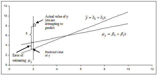
Figure \(\PageIndex{5}\). Illustrating the two components in the error of prediction.
The variance of the difference between y and \(\hat y\) is the sum of these two variances and forms the basis for the standard error of \((y-\hat y)\) used for prediction. The resulting form of a prediction interval is as follows:
\[\]\hat y \pm t_{\alpha/2}s\sqrt {1+\frac {1}{n} + \frac {(x_0 - \bar x)^2}{\sum (x_i - \bar x)^2}} \]
where x0 is the given value for the predictor variable, n is the number of observations, and \(t_{\alpha/2}\) is the critical value with (n – 2) degrees of freedom.
Software, such as Minitab, can compute the prediction intervals. Using the data from the previous example, we will use Minitab to compute the 95% prediction interval for the IBI of a specific forested area of 32 km.
|
Predicted Values for New Observations |
|||
|
New Obs |
Fit |
SE Fit |
95% PI |
|
1 |
49.9496 |
2.38400 |
(20.1053, 79.7939) |
You can repeat this process many times for several different values of x and plot the prediction intervals for the mean response.
|
x |
95% PI |
|
20 |
(13.01, 73.11) |
|
40 |
(24.77, 84.31) |
|
60 |
(36.21, 95.83) |
|
80 |
(47.33, 107.67) |
|
100 |
(58.15, 119.81) |
Notice that the prediction interval bands are wider than the corresponding confidence interval bands, reflecting the fact that we are predicting the value of a random variable rather than estimating a population parameter. We would expect predictions for an individual value to be more variable than estimates of an average value.
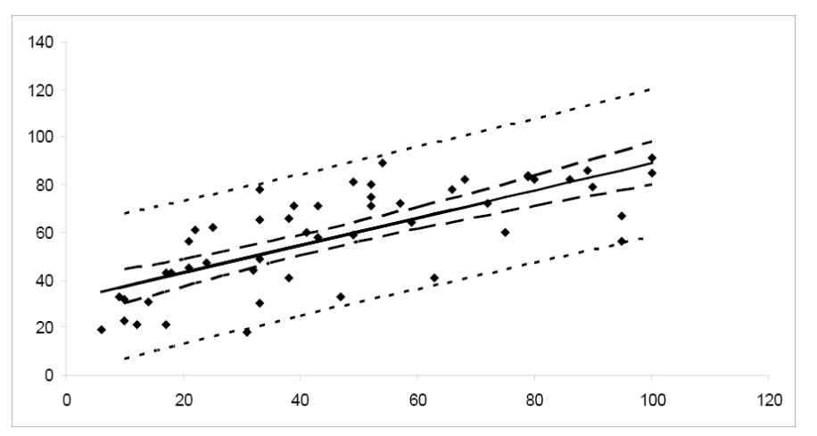
Figure \(\PageIndex{6}\). A comparison of confidence and prediction intervals.
Transformations to Linearize Data Relationships
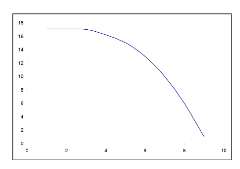
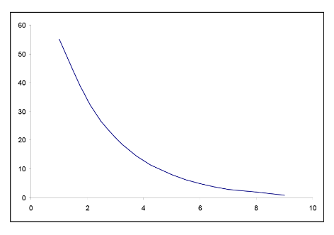
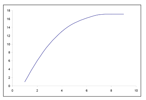
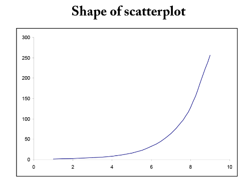
In many situations, the relationship between x and y is non-linear. In order to simplify the underlying model, we can transform or convert either x or y or both to result in a more linear relationship. There are many common transformations such as logarithmic and reciprocal. Including higher order terms on x may also help to linearize the relationship between x and y. Shown below are some common shapes of scatterplots and possible choices for transformations. However, the choice of transformation is frequently more a matter of trial and error than set rules.
 |
\[ \begin{array}{lll} |
 |
\[ \begin{array}{lll} |
 |
\[ \begin{array}{lll} |
 |
Choice of transformation \[ \begin{array}{lll} |
Figure \(\PageIndex{7}\). Examples of possible transformations for x and y variables.
A forester needs to create a simple linear regression model to predict tree volume using diameter-at-breast height (dbh) for sugar maple trees. He collects dbh and volume for 236 sugar maple trees and plots volume versus dbh. Given below is the scatterplot, correlation coefficient, and regression output from Minitab.
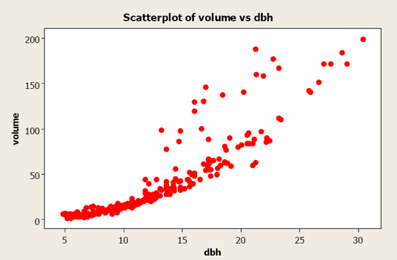
Figure \(\PageIndex{8}\) Scatterplot of volume versus dbh.
Pearson’s linear correlation coefficient is 0.894, which indicates a strong, positive, linear relationship. However, the scatterplot shows a distinct nonlinear relationship.
Regression Analysis: volume versus dbh
| The regression equation is volume = – 51.1 + 7.15 dbh | ||||
|
Predictor |
Coef |
SE Coef |
T |
P |
|
Constant |
-51.097 |
3.271 |
-15.62 |
0.000 |
|
dbh |
7.1500 |
0.2342 |
30.53 |
0.000 |
|
S = 19.5820 |
R-Sq = 79.9% |
R-Sq(adj) = 79.8% |
||
|
Analysis of Variance |
|||||
|
Source |
DF |
SS |
MS |
F |
P |
|
Regression |
1 |
357397 |
357397 |
932.04 |
0.000 |
|
Residual Error |
234 |
89728 |
383 |
||
|
Total |
235 |
447125 |
|||
The R2 is 79.9% indicating a fairly strong model and the slope is significantly different from zero. However, both the residual plot and the residual normal probability plot indicate serious problems with this model. A transformation may help to create a more linear relationship between volume and dbh.

Figure \(\PageIndex{9}\). Residual and normal probability plots.
Volume was transformed to the natural log of volume and plotted against dbh (see scatterplot below). Unfortunately, this did little to improve the linearity of this relationship. The forester then took the natural log transformation of dbh. The scatterplot of the natural log of volume versus the natural log of dbh indicated a more linear relationship between these two variables. The linear correlation coefficient is 0.954.
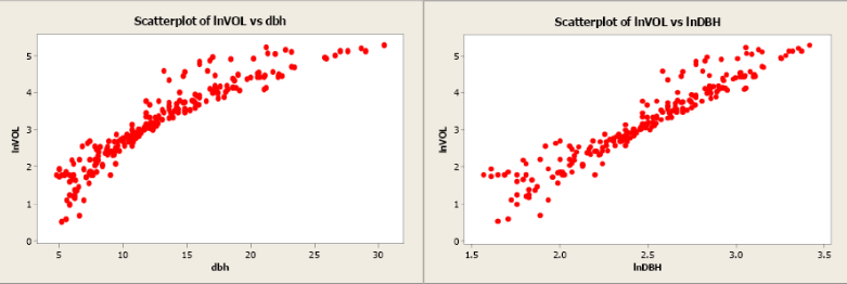
Figure \(\PageIndex{10}\). Scatterplots of natural log of volume versus dbh and natural log of volume versus natural log of dbh.
The regression analysis output from Minitab is given below.
Regression Analysis: lnVOL vs. lnDBH
|
The regression equation is lnVOL = – 2.86 + 2.44 lnDBH |
||||
|
Predictor |
Coef |
SE Coef |
T |
P |
|
Constant |
-2.8571 |
0.1253 |
-22.80 |
0.000 |
|
lnDBH |
2.44383 |
0.05007 |
48.80 |
0.000 |
|
S = 0.327327 |
R-Sq = 91.1% |
R-Sq(adj) = 91.0% |
||
|
Analysis of Variance |
|||||
|
Source |
DF |
SS |
MS |
F |
P |
|
Regression |
1 |
255.19 |
255.19 |
2381.78 |
0.000 |
|
Residual Error |
234 |
25.07 |
0.11 |
||
|
Total |
235 |
280.26 |
|||

Figure \(\PageIndex{11}\). Residual and normal probability plots.
The model using the transformed values of volume and dbh has a more linear relationship and a more positive correlation coefficient. The slope is significantly different from zero and the R2 has increased from 79.9% to 91.1%. The residual plot shows a more random pattern and the normal probability plot shows some improvement.
There are many possible transformation combinations possible to linearize data. Each situation is unique and the user may need to try several alternatives before selecting the best transformation for x or y or both.


