
6.3: Summary And Software Solution
- Page ID
- 2906

\( \newcommand{\vecs}[1]{\overset { \scriptstyle \rightharpoonup} {\mathbf{#1}} } \)
\( \newcommand{\vecd}[1]{\overset{-\!-\!\rightharpoonup}{\vphantom{a}\smash {#1}}} \)
\( \newcommand{\dsum}{\displaystyle\sum\limits} \)
\( \newcommand{\dint}{\displaystyle\int\limits} \)
\( \newcommand{\dlim}{\displaystyle\lim\limits} \)
\( \newcommand{\id}{\mathrm{id}}\) \( \newcommand{\Span}{\mathrm{span}}\)
( \newcommand{\kernel}{\mathrm{null}\,}\) \( \newcommand{\range}{\mathrm{range}\,}\)
\( \newcommand{\RealPart}{\mathrm{Re}}\) \( \newcommand{\ImaginaryPart}{\mathrm{Im}}\)
\( \newcommand{\Argument}{\mathrm{Arg}}\) \( \newcommand{\norm}[1]{\| #1 \|}\)
\( \newcommand{\inner}[2]{\langle #1, #2 \rangle}\)
\( \newcommand{\Span}{\mathrm{span}}\)
\( \newcommand{\id}{\mathrm{id}}\)
\( \newcommand{\Span}{\mathrm{span}}\)
\( \newcommand{\kernel}{\mathrm{null}\,}\)
\( \newcommand{\range}{\mathrm{range}\,}\)
\( \newcommand{\RealPart}{\mathrm{Re}}\)
\( \newcommand{\ImaginaryPart}{\mathrm{Im}}\)
\( \newcommand{\Argument}{\mathrm{Arg}}\)
\( \newcommand{\norm}[1]{\| #1 \|}\)
\( \newcommand{\inner}[2]{\langle #1, #2 \rangle}\)
\( \newcommand{\Span}{\mathrm{span}}\) \( \newcommand{\AA}{\unicode[.8,0]{x212B}}\)
\( \newcommand{\vectorA}[1]{\vec{#1}} % arrow\)
\( \newcommand{\vectorAt}[1]{\vec{\text{#1}}} % arrow\)
\( \newcommand{\vectorB}[1]{\overset { \scriptstyle \rightharpoonup} {\mathbf{#1}} } \)
\( \newcommand{\vectorC}[1]{\textbf{#1}} \)
\( \newcommand{\vectorD}[1]{\overrightarrow{#1}} \)
\( \newcommand{\vectorDt}[1]{\overrightarrow{\text{#1}}} \)
\( \newcommand{\vectE}[1]{\overset{-\!-\!\rightharpoonup}{\vphantom{a}\smash{\mathbf {#1}}}} \)
\( \newcommand{\vecs}[1]{\overset { \scriptstyle \rightharpoonup} {\mathbf{#1}} } \)
\(\newcommand{\longvect}{\overrightarrow}\)
\( \newcommand{\vecd}[1]{\overset{-\!-\!\rightharpoonup}{\vphantom{a}\smash {#1}}} \)
\(\newcommand{\avec}{\mathbf a}\) \(\newcommand{\bvec}{\mathbf b}\) \(\newcommand{\cvec}{\mathbf c}\) \(\newcommand{\dvec}{\mathbf d}\) \(\newcommand{\dtil}{\widetilde{\mathbf d}}\) \(\newcommand{\evec}{\mathbf e}\) \(\newcommand{\fvec}{\mathbf f}\) \(\newcommand{\nvec}{\mathbf n}\) \(\newcommand{\pvec}{\mathbf p}\) \(\newcommand{\qvec}{\mathbf q}\) \(\newcommand{\svec}{\mathbf s}\) \(\newcommand{\tvec}{\mathbf t}\) \(\newcommand{\uvec}{\mathbf u}\) \(\newcommand{\vvec}{\mathbf v}\) \(\newcommand{\wvec}{\mathbf w}\) \(\newcommand{\xvec}{\mathbf x}\) \(\newcommand{\yvec}{\mathbf y}\) \(\newcommand{\zvec}{\mathbf z}\) \(\newcommand{\rvec}{\mathbf r}\) \(\newcommand{\mvec}{\mathbf m}\) \(\newcommand{\zerovec}{\mathbf 0}\) \(\newcommand{\onevec}{\mathbf 1}\) \(\newcommand{\real}{\mathbb R}\) \(\newcommand{\twovec}[2]{\left[\begin{array}{r}#1 \\ #2 \end{array}\right]}\) \(\newcommand{\ctwovec}[2]{\left[\begin{array}{c}#1 \\ #2 \end{array}\right]}\) \(\newcommand{\threevec}[3]{\left[\begin{array}{r}#1 \\ #2 \\ #3 \end{array}\right]}\) \(\newcommand{\cthreevec}[3]{\left[\begin{array}{c}#1 \\ #2 \\ #3 \end{array}\right]}\) \(\newcommand{\fourvec}[4]{\left[\begin{array}{r}#1 \\ #2 \\ #3 \\ #4 \end{array}\right]}\) \(\newcommand{\cfourvec}[4]{\left[\begin{array}{c}#1 \\ #2 \\ #3 \\ #4 \end{array}\right]}\) \(\newcommand{\fivevec}[5]{\left[\begin{array}{r}#1 \\ #2 \\ #3 \\ #4 \\ #5 \\ \end{array}\right]}\) \(\newcommand{\cfivevec}[5]{\left[\begin{array}{c}#1 \\ #2 \\ #3 \\ #4 \\ #5 \\ \end{array}\right]}\) \(\newcommand{\mattwo}[4]{\left[\begin{array}{rr}#1 \amp #2 \\ #3 \amp #4 \\ \end{array}\right]}\) \(\newcommand{\laspan}[1]{\text{Span}\{#1\}}\) \(\newcommand{\bcal}{\cal B}\) \(\newcommand{\ccal}{\cal C}\) \(\newcommand{\scal}{\cal S}\) \(\newcommand{\wcal}{\cal W}\) \(\newcommand{\ecal}{\cal E}\) \(\newcommand{\coords}[2]{\left\{#1\right\}_{#2}}\) \(\newcommand{\gray}[1]{\color{gray}{#1}}\) \(\newcommand{\lgray}[1]{\color{lightgray}{#1}}\) \(\newcommand{\rank}{\operatorname{rank}}\) \(\newcommand{\row}{\text{Row}}\) \(\newcommand{\col}{\text{Col}}\) \(\renewcommand{\row}{\text{Row}}\) \(\newcommand{\nul}{\text{Nul}}\) \(\newcommand{\var}{\text{Var}}\) \(\newcommand{\corr}{\text{corr}}\) \(\newcommand{\len}[1]{\left|#1\right|}\) \(\newcommand{\bbar}{\overline{\bvec}}\) \(\newcommand{\bhat}{\widehat{\bvec}}\) \(\newcommand{\bperp}{\bvec^\perp}\) \(\newcommand{\xhat}{\widehat{\xvec}}\) \(\newcommand{\vhat}{\widehat{\vvec}}\) \(\newcommand{\uhat}{\widehat{\uvec}}\) \(\newcommand{\what}{\widehat{\wvec}}\) \(\newcommand{\Sighat}{\widehat{\Sigma}}\) \(\newcommand{\lt}{<}\) \(\newcommand{\gt}{>}\) \(\newcommand{\amp}{&}\) \(\definecolor{fillinmathshade}{gray}{0.9}\)Summary
Two-way analysis of variance allows you to examine the effect of two factors simultaneously on the average response. The interaction of these two factors is always the starting point for two-way ANOVA. If the interaction term is significant, then you will ignore the main effects and focus solely on the unique treatments (combinations of the different levels of the two factors). If the interaction term is not significant, then it is appropriate to investigate the presence of the main effect of the response variable separately.
Software Solutions
Minitab
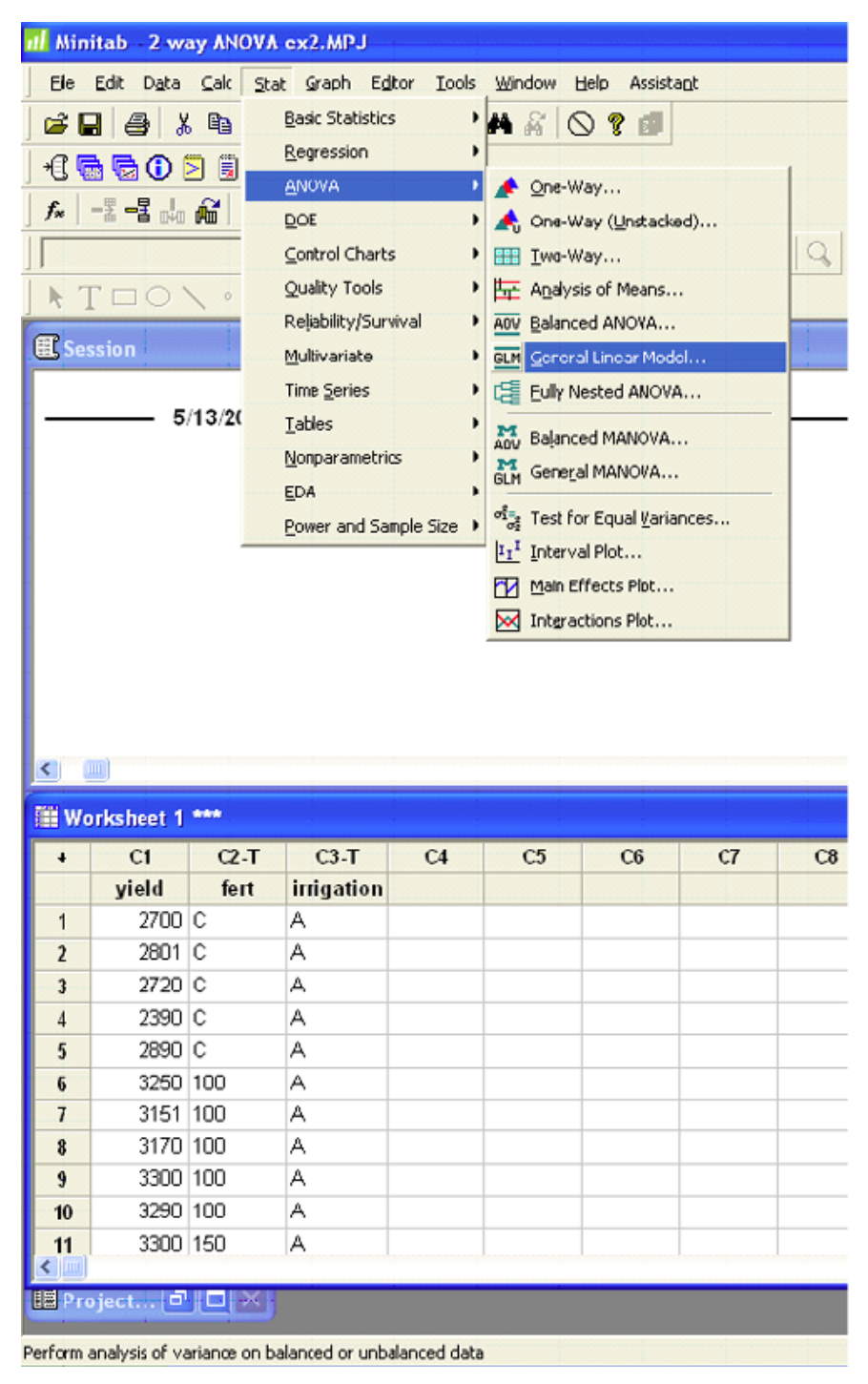
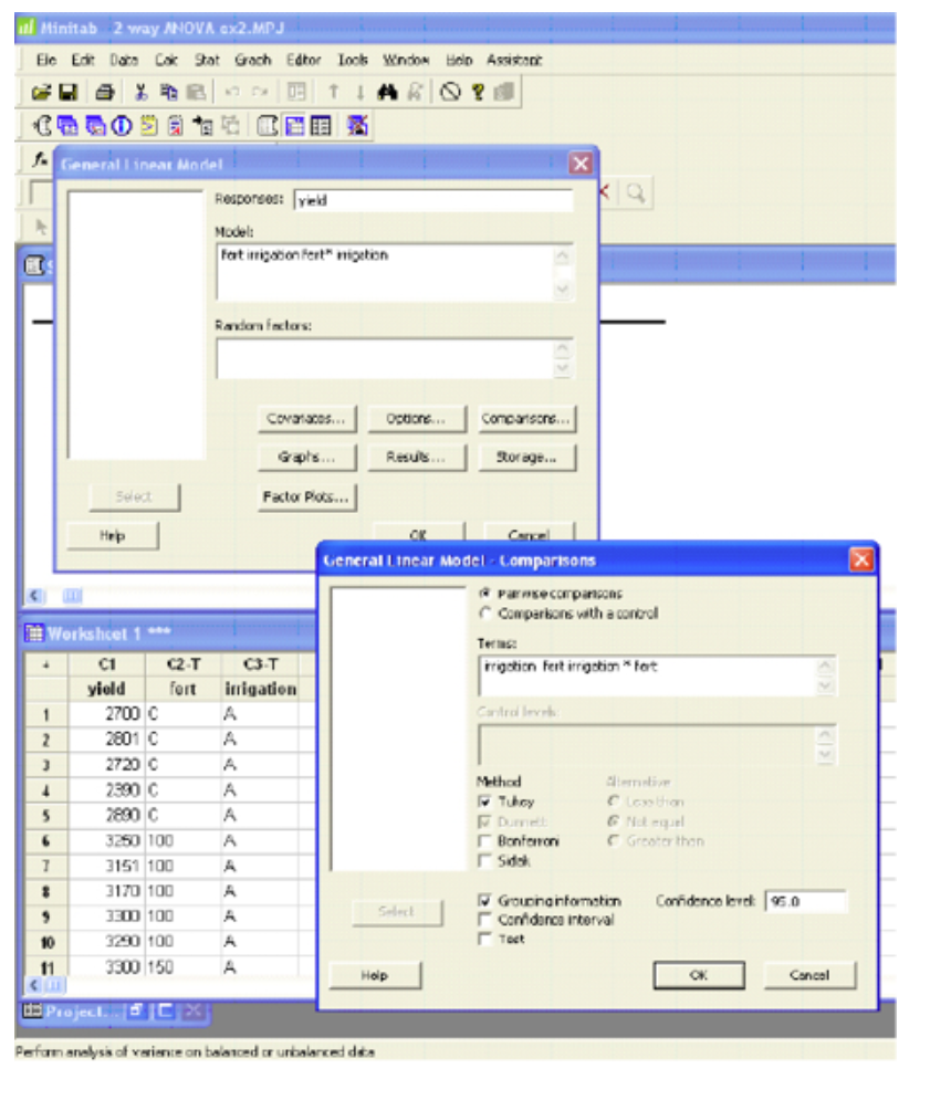
General Linear Model: yield vs. fert, irrigation
|
Factor |
Type |
Levels |
Values |
|||
|
fert |
fixed |
4 |
100, |
150, |
200, |
C |
|
irrigation |
fixed |
4 |
A, |
B, |
C, |
D |
|
Analysis of Variance for Yield, using Adjusted SS for Tests |
||||||
|
Source |
DF |
Seq SS |
Adj SS |
Adj MS |
F |
P |
|
fert |
3 |
1128272 |
1128272 |
376091 |
12.76 |
0.000 |
|
irrigation |
3 |
161776127 |
161776127 |
53925376 |
1830.16 |
0.000 |
|
fert*irrigation |
9 |
2088667 |
2088667 |
232074 |
7.88 |
0.000 |
|
Error |
64 |
1885746 |
1885746 |
29465 |
||
|
Total |
79 |
166878812 |
||||
|
S = 171.653 R-Sq = 98.87% R-Sq(adj) = 98.61% |
||||||
|
Unusual Observations for yield |
|||||||
|
Obs |
yield |
Fit |
SE |
Fit |
Residual |
St |
Resid |
|
4 |
2390.00 |
2700.20 |
76.77 |
-310.20 |
-2.02 |
R |
|
|
28 |
2250.00 |
2646.00 |
76.77 |
-396.00 |
-2.58 |
R |
|
|
35 |
4250.00 |
3327.60 |
76.77 |
922.40 |
6.01 |
R |
|
|
R denotes an observation with a large standardized residual. |
|||||||
|
Grouping Information Using Tukey Method and 95.0% Confidence |
|||||||
|
irrigation |
N |
Mean |
Grouping |
||||
|
A |
20 |
3120.60 |
A |
||||
|
B |
20 |
3040.05 |
A |
||||
|
C |
20 |
352.85 |
B |
||||
|
D |
20 |
129.55 |
C |
||||
|
Means that do not share a letter are significantly different. |
|||||||
|
Grouping Information Using Tukey Method and 95.0% Confidence |
|||||||
|
fert |
N |
Mean |
Grouping |
||||
|
150 |
20 |
1797.90 |
A |
||||
|
200 |
20 |
1749.95 |
A |
||||
|
100 |
20 |
1592.55 |
B |
||||
|
C |
20 |
1502.65 |
B |
||||
|
Means that do not share a letter are significantly different. |
|||||||
|
Grouping Information Using Tukey Method and 95.0% Confidence |
|||||||
|
fert |
irrigation |
N |
Mean |
Grouping |
|||
|
200 |
A |
5 |
3381.00 |
A |
|||
|
150 |
B |
5 |
3327.60 |
A |
|||
|
100 |
A |
5 |
3232.20 |
A |
|||
|
150 |
A |
5 |
3169.00 |
A |
|||
|
200 |
B |
5 |
3097.00 |
A |
|||
|
C |
B |
5 |
3089.60 |
A |
|||
|
C |
A |
5 |
2700.20 |
B |
|||
|
100 |
B |
5 |
2646.00 |
B |
|||
|
150 |
C |
5 |
623.80 |
C |
|||
|
100 |
C |
5 |
340.60 |
C |
D |
||
|
200 |
C |
5 |
338.00 |
C |
D |
||
|
200 |
D |
5 |
183.80 |
D |
|||
|
100 |
D |
5 |
151.40 |
D |
|||
|
C |
D |
5 |
111.80 |
D |
|||
|
C |
C |
5 |
109.00 |
D |
|||
|
150 |
D |
5 |
71.20 |
D |
|||
|
Means that do not share a letter are significantly different. |
|||||||
Excel
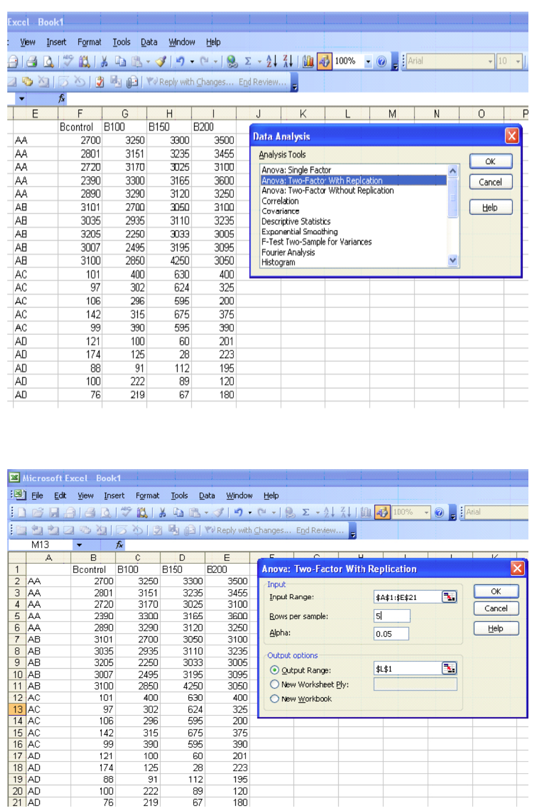
|
Anova: Two-Factor With Replication |
||||||
|
SUMMARY |
Bcontrol |
B100 |
B150 |
B200 |
Total |
|
|
AA |
||||||
|
Count |
5 |
5 |
5 |
5 |
20 |
|
|
Sum |
13501 |
16161 |
15845 |
16905 |
62412 |
|
|
Average |
2700.2 |
3232.2 |
3169 |
3381 |
3120.6 |
|
|
Variance |
35700.2 |
4679.2 |
11167.5 |
40930 |
87716.57 |
|
|
AB |
||||||
|
Count |
5 |
5 |
5 |
5 |
20 |
|
|
Sum |
15448 |
13230 |
16638 |
15485 |
60801 |
|
|
Average |
3089.6 |
2646 |
3327.6 |
3097 |
3040.05 |
|
|
Variance |
5839.8 |
76917.5 |
269901.3 |
7432.5 |
139929.4 |
|
|
AC |
||||||
|
Count |
5 |
5 |
5 |
5 |
20 |
|
|
Sum |
545 |
1703 |
3119 |
1690 |
7057 |
|
|
Average |
109 |
340.6 |
623.8 |
338 |
352.85 |
|
|
Variance |
351.5 |
2525.8 |
1079.7 |
6782.5 |
37326.03 |
|
|
AD |
||||||
|
Count |
5 |
5 |
5 |
5 |
20 |
|
|
Sum |
559 |
757 |
356 |
919 |
2591 |
|
|
Average |
111.8 |
151.4 |
71.2 |
183.8 |
129.55 |
|
|
Variance |
1485.2 |
4135.3 |
997.7 |
1510.7 |
3590.366 |
|
|
Total |
||||||
|
Count |
20 |
20 |
20 |
20 |
||
|
Sum |
30053 |
31851 |
35958 |
34999 |
||
|
Average |
1502.65 |
1592.55 |
1797.9 |
1749.95 |
||
|
Variance |
2069464 |
1977134 |
2317478 |
2359637 |
||
|
ANOVA |
||||||
|
Source of Variation |
SS |
df |
MS |
F |
p-value |
F crit |
|
Sample |
1.62E+08 |
3 |
53925376 |
1830.164 |
5.98E-62 |
2.748191 |
|
Columns |
1128272 |
3 |
376090.7 |
12.76408 |
1.23E-06 |
2.748191 |
|
Interaction |
2088667 |
9 |
232074.2 |
7.876325 |
1.02E-07 |
2.029792 |
|
Within |
1885746 |
64 |
29464.78 |
|||
|
Total |
1.67E+08 |
79 |
||||