6.2: Multiple Comparisons
- Page ID
- 2905

\( \newcommand{\vecs}[1]{\overset { \scriptstyle \rightharpoonup} {\mathbf{#1}} } \)
\( \newcommand{\vecd}[1]{\overset{-\!-\!\rightharpoonup}{\vphantom{a}\smash {#1}}} \)
\( \newcommand{\id}{\mathrm{id}}\) \( \newcommand{\Span}{\mathrm{span}}\)
( \newcommand{\kernel}{\mathrm{null}\,}\) \( \newcommand{\range}{\mathrm{range}\,}\)
\( \newcommand{\RealPart}{\mathrm{Re}}\) \( \newcommand{\ImaginaryPart}{\mathrm{Im}}\)
\( \newcommand{\Argument}{\mathrm{Arg}}\) \( \newcommand{\norm}[1]{\| #1 \|}\)
\( \newcommand{\inner}[2]{\langle #1, #2 \rangle}\)
\( \newcommand{\Span}{\mathrm{span}}\)
\( \newcommand{\id}{\mathrm{id}}\)
\( \newcommand{\Span}{\mathrm{span}}\)
\( \newcommand{\kernel}{\mathrm{null}\,}\)
\( \newcommand{\range}{\mathrm{range}\,}\)
\( \newcommand{\RealPart}{\mathrm{Re}}\)
\( \newcommand{\ImaginaryPart}{\mathrm{Im}}\)
\( \newcommand{\Argument}{\mathrm{Arg}}\)
\( \newcommand{\norm}[1]{\| #1 \|}\)
\( \newcommand{\inner}[2]{\langle #1, #2 \rangle}\)
\( \newcommand{\Span}{\mathrm{span}}\) \( \newcommand{\AA}{\unicode[.8,0]{x212B}}\)
\( \newcommand{\vectorA}[1]{\vec{#1}} % arrow\)
\( \newcommand{\vectorAt}[1]{\vec{\text{#1}}} % arrow\)
\( \newcommand{\vectorB}[1]{\overset { \scriptstyle \rightharpoonup} {\mathbf{#1}} } \)
\( \newcommand{\vectorC}[1]{\textbf{#1}} \)
\( \newcommand{\vectorD}[1]{\overrightarrow{#1}} \)
\( \newcommand{\vectorDt}[1]{\overrightarrow{\text{#1}}} \)
\( \newcommand{\vectE}[1]{\overset{-\!-\!\rightharpoonup}{\vphantom{a}\smash{\mathbf {#1}}}} \)
\( \newcommand{\vecs}[1]{\overset { \scriptstyle \rightharpoonup} {\mathbf{#1}} } \)
\( \newcommand{\vecd}[1]{\overset{-\!-\!\rightharpoonup}{\vphantom{a}\smash {#1}}} \)
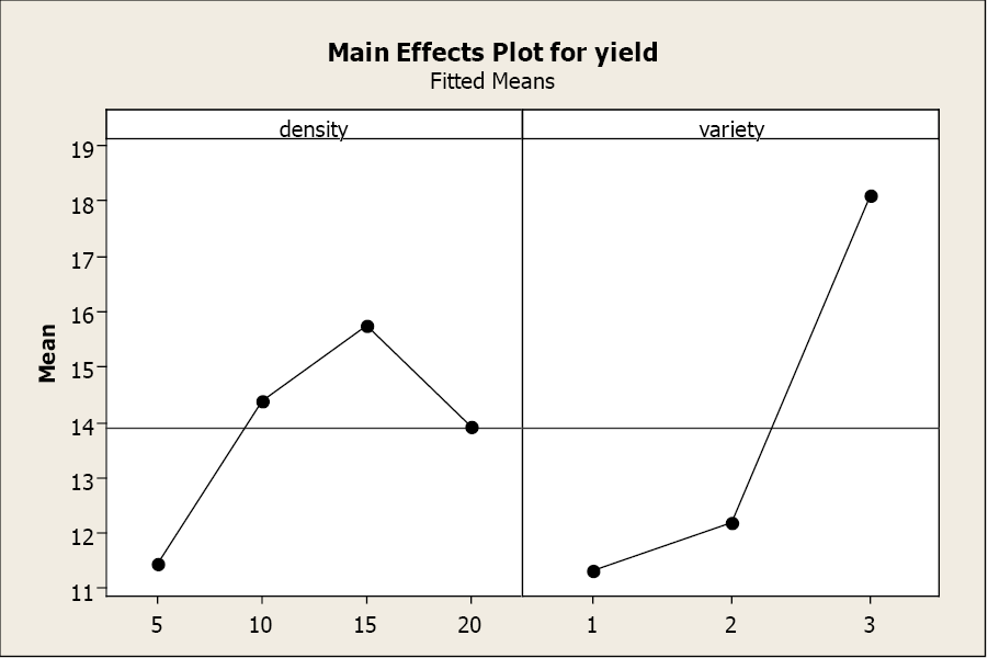
\(\newcommand{\avec}{\mathbf a}\) \(\newcommand{\bvec}{\mathbf b}\) \(\newcommand{\cvec}{\mathbf c}\) \(\newcommand{\dvec}{\mathbf d}\) \(\newcommand{\dtil}{\widetilde{\mathbf d}}\) \(\newcommand{\evec}{\mathbf e}\) \(\newcommand{\fvec}{\mathbf f}\) \(\newcommand{\nvec}{\mathbf n}\) \(\newcommand{\pvec}{\mathbf p}\) \(\newcommand{\qvec}{\mathbf q}\) \(\newcommand{\svec}{\mathbf s}\) \(\newcommand{\tvec}{\mathbf t}\) \(\newcommand{\uvec}{\mathbf u}\) \(\newcommand{\vvec}{\mathbf v}\) \(\newcommand{\wvec}{\mathbf w}\) \(\newcommand{\xvec}{\mathbf x}\) \(\newcommand{\yvec}{\mathbf y}\) \(\newcommand{\zvec}{\mathbf z}\) \(\newcommand{\rvec}{\mathbf r}\) \(\newcommand{\mvec}{\mathbf m}\) \(\newcommand{\zerovec}{\mathbf 0}\) \(\newcommand{\onevec}{\mathbf 1}\) \(\newcommand{\real}{\mathbb R}\) \(\newcommand{\twovec}[2]{\left[\begin{array}{r}#1 \\ #2 \end{array}\right]}\) \(\newcommand{\ctwovec}[2]{\left[\begin{array}{c}#1 \\ #2 \end{array}\right]}\) \(\newcommand{\threevec}[3]{\left[\begin{array}{r}#1 \\ #2 \\ #3 \end{array}\right]}\) \(\newcommand{\cthreevec}[3]{\left[\begin{array}{c}#1 \\ #2 \\ #3 \end{array}\right]}\) \(\newcommand{\fourvec}[4]{\left[\begin{array}{r}#1 \\ #2 \\ #3 \\ #4 \end{array}\right]}\) \(\newcommand{\cfourvec}[4]{\left[\begin{array}{c}#1 \\ #2 \\ #3 \\ #4 \end{array}\right]}\) \(\newcommand{\fivevec}[5]{\left[\begin{array}{r}#1 \\ #2 \\ #3 \\ #4 \\ #5 \\ \end{array}\right]}\) \(\newcommand{\cfivevec}[5]{\left[\begin{array}{c}#1 \\ #2 \\ #3 \\ #4 \\ #5 \\ \end{array}\right]}\) \(\newcommand{\mattwo}[4]{\left[\begin{array}{rr}#1 \amp #2 \\ #3 \amp #4 \\ \end{array}\right]}\) \(\newcommand{\laspan}[1]{\text{Span}\{#1\}}\) \(\newcommand{\bcal}{\cal B}\) \(\newcommand{\ccal}{\cal C}\) \(\newcommand{\scal}{\cal S}\) \(\newcommand{\wcal}{\cal W}\) \(\newcommand{\ecal}{\cal E}\) \(\newcommand{\coords}[2]{\left\{#1\right\}_{#2}}\) \(\newcommand{\gray}[1]{\color{gray}{#1}}\) \(\newcommand{\lgray}[1]{\color{lightgray}{#1}}\) \(\newcommand{\rank}{\operatorname{rank}}\) \(\newcommand{\row}{\text{Row}}\) \(\newcommand{\col}{\text{Col}}\) \(\renewcommand{\row}{\text{Row}}\) \(\newcommand{\nul}{\text{Nul}}\) \(\newcommand{\var}{\text{Var}}\) \(\newcommand{\corr}{\text{corr}}\) \(\newcommand{\len}[1]{\left|#1\right|}\) \(\newcommand{\bbar}{\overline{\bvec}}\) \(\newcommand{\bhat}{\widehat{\bvec}}\) \(\newcommand{\bperp}{\bvec^\perp}\) \(\newcommand{\xhat}{\widehat{\xvec}}\) \(\newcommand{\vhat}{\widehat{\vvec}}\) \(\newcommand{\uhat}{\widehat{\uvec}}\) \(\newcommand{\what}{\widehat{\wvec}}\) \(\newcommand{\Sighat}{\widehat{\Sigma}}\) \(\newcommand{\lt}{<}\) \(\newcommand{\gt}{>}\) \(\newcommand{\amp}{&}\) \(\definecolor{fillinmathshade}{gray}{0.9}\)The next step is to examine the multiple comparisons for each main effect to determine the differences. We will proceed as we did with one-way ANOVA multiple comparisons by examining the Tukey’s Grouping for each main effect. For factor A, variety, the sample means, and grouping letters are presented to identify those varieties that are significantly different from other varieties. Varieties 1 and 2 are not significantly different from each other, both producing similar yields. Variety 3 produced significantly greater yields than both variety 1 and 2.
Grouping Information Using Tukey Method and 95.0% Confidence
|
variety |
N |
Mean |
Grouping |
|
|---|---|---|---|---|
|
3 |
12 |
18.117 |
A |
|
|
2 |
12 |
12.208 |
B |
|
|
1 |
12 |
11.317 |
B |
|
|
Means that do not share a letter are significantly different. |
||||
Some of the densities are also significantly different. We will follow the same procedure to determine the differences.
Grouping Information Using Tukey Method and 95.0% Confidence
|
density |
N |
Mean |
Grouping |
||
|---|---|---|---|---|---|
|
15 |
9 |
15.756 |
A |
||
|
10 |
9 |
14.389 |
A |
B |
|
|
20 |
9 |
13.922 |
B |
||
|
5 |
9 |
11.456 |
C |
||
|
Means that do not share a letter are significantly different. |
|||||
The Grouping Information shows us that a planting density of 15,000 plants/plot results in the greatest yield. However, there is no significant difference in yield between 10,000 and 15,000 plants/plot or between 10,000 and 20,000 plants/plot. The plots with 5,000 plants/plot result in the lowest yields and these yields are significantly lower than all other densities tested.
The main effects plots also illustrate the differences in yield across the three varieties and four densities.
But what happens if there is a significant interaction between the main effects? This next example will demonstrate how a significant interaction alters the interpretation of a 2-way ANOVA.
A researcher was interested in the effects of four levels of fertilization (control, 100 lb., 150 lb., and 200 lb.) and four levels of irrigation (A, B, C, and D) on biomass yield. The sixteen possible treatment combinations were randomly assigned to 80 plots (5 plots for each treatment). The total biomass yields for each treatment are listed below.
|
Fertilizer |
||||
|
Irrigation |
Control |
100 lb. |
150 lb. |
200 lb. |
|
A |
2700,2801,2720, 2390, 2890 |
3250, 3151, 3170, 3300, 3290 |
3300, 3235, 3025, 3165, 3120 |
3500, 3455, 3100, 3600, 3250 |
|
B |
3101, 3035, 3205, 3007, 3100 |
2700, 2935, 2250, 2495, 2850 |
3050, 3110, 3033, 3195, 4250 |
3100, 3235, 3005, 3095, 3050 |
|
C |
101, 97, 106, 142, 99 |
400, 302, 296, 315, 390 |
630, 624, 595, 675, 595 |
400, 325, 200, 375, 390 |
|
D |
121, 174, 88, 100, 76 |
100, 125, 91, 222, 219 |
60, 28, 112, 89, 67 |
201, 223, 195, 120, 180 |
Table 6. Observed data for four irrigation levels and four fertilizer levels.
Factor A (irrigation level) has k = 4 levels and factor B (fertilizer) has l = 4 levels. There are m = 5 replicates and 80 total observations. This is a balanced design as the number of replicates is equal. The ANOVA table is presented next.
Two-way ANOVA table.
|
Source |
DF |
SS |
MSS |
F |
P |
|
fertilizer |
3 |
1128272 |
376091 |
12.76 |
<0.001 |
|
irrigation |
3 |
161776127 |
53925376 |
1830.16 |
<0.001 |
|
fert*irrigation |
9 |
2088667 |
232074 |
7.88 |
<0.001 |
|
error |
64 |
1885746 |
29465 |
||
|
total |
79 |
166878812 |
We again begin with testing the interaction term. Remember, if the interaction term is significant, we ignore the main effects.
\(H_0\): There is no interaction between factors
\(H_1\): There is a significant interaction between factors
The F-statistic:
\[F_{AB} = \dfrac {MSAB}{MSE} = \dfrac {232074}{29465} = 7.88 \nonumber \]
The p-value for the test for a significant interaction between factors is <0.001. This p-value is less than 5%, therefore we reject the null hypothesis. There is evidence of a significant interaction between fertilizer and irrigation. Since the interaction term is significant, we do not investigate the presence of the main effects. We must now examine multiple comparisons for all 16 treatments (each combination of fertilizer and irrigation level) to determine the differences in yield, aided by the factor plot.
Grouping Information Using Tukey Method and 95.0% Confidence
|
fert |
irrigation |
N |
Mean |
Grouping |
|||
|
200 |
A |
5 |
3381.00 |
A |
|||
|
150 |
B |
5 |
3327.60 |
A |
|||
|
100 |
A |
5 |
3232.20 |
A |
|||
|
150 |
A |
5 |
3169.00 |
A |
|||
|
200 |
B |
5 |
3097.00 |
A |
|||
|
C |
B |
5 |
3089.60 |
A |
|||
|
C |
A |
5 |
2700.20 |
B |
|||
|
100 |
B |
5 |
2646.00 |
B |
|||
|
150 |
C |
5 |
623.80 |
C |
|||
|
100 |
C |
5 |
340.60 |
C |
D |
||
|
200 |
C |
5 |
338.00 |
C |
D |
||
|
200 |
D |
5 |
183.80 |
D |
|||
|
100 |
D |
5 |
151.40 |
D |
|||
|
C |
D |
5 |
111.80 |
D |
|||
|
C |
C |
5 |
109.00 |
D |
|||
|
150 |
D |
5 |
71.20 |
D |
|||
|
Means that do not share a letter are significantly different. |
|||||||
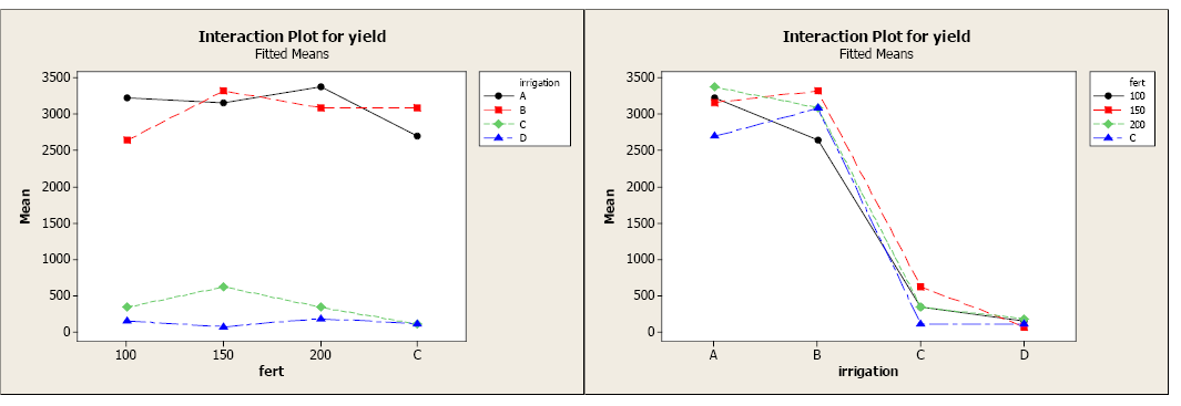
The factor plot allows you to visualize the differences between the 16 treatments. Factor plots can present the information two ways, each with a different factor on the x-axis. In the first plot, fertilizer level is on the x-axis. There is a clear distinction in average yields for the different treatments. Irrigation levels A and B appear to be producing greater yields across all levels of fertilizers compared to irrigation levels C and D. In the second plot, irrigation level is on the x-axis. All levels of fertilizer seem to result in greater yields for irrigation levels A and B compared to C and D.
The next step is to use the multiple comparison output to determine where there are SIGNIFICANT differences. Let’s focus on the first factor plot to do this.
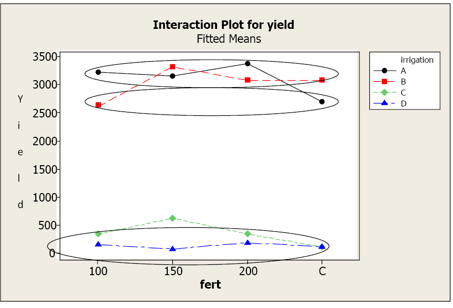
The Grouping Information tells us that while irrigation levels A and B look similar across all levels of fertilizer, only treatments A-100, A-150, A-200, B-control, B-150, and B-200 are statistically similar (upper circle). Treatment B-100 and A-control also result in similar yields (middle circle) and both have significantly lower yields than the first group.
Irrigation levels C and D result in the lowest yields across the fertilizer levels. We again refer to the Grouping Information to identify the differences. There is no significant difference in yield for irrigation level D over any level of fertilizer. Yields for D are also similar to yields for irrigation level C at 100, 200, and control levels for fertilizer (lowest circle). Irrigation level C at 150 level fertilizer results in significantly higher yields than any yield from irrigation level D for any fertilizer level, however, this yield is still significantly smaller than the first group using irrigation levels A and B.
Interpreting Factor Plots
When the interaction term is significant the analysis focuses solely on the treatments, not the main effects. The factor plot and grouping information allow the researcher to identify similarities and differences, along with any trends or patterns. The following series of factor plots illustrate some true average responses in terms of interactions and main effects.
This first plot clearly shows a significant interaction between the factors. The change in response when level B changes, depends on level A.
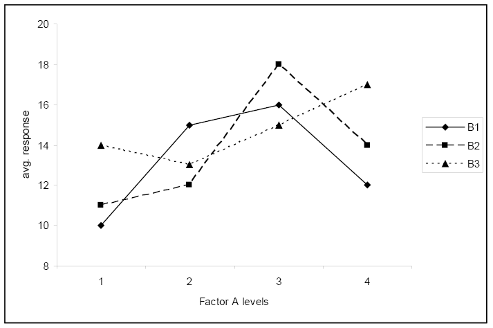

Figure 5.
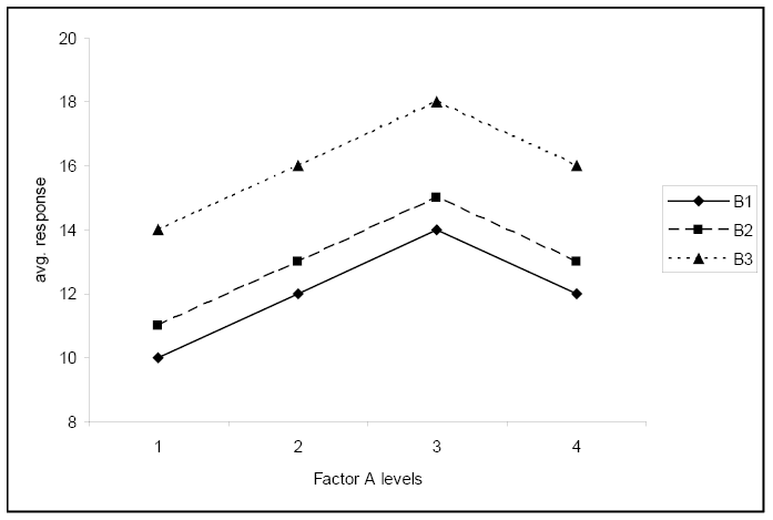
The second plot shows no significant interaction. The change in response for the level of factor A is the same for each level of factor B.
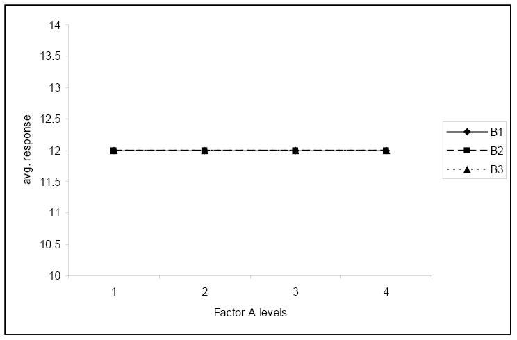
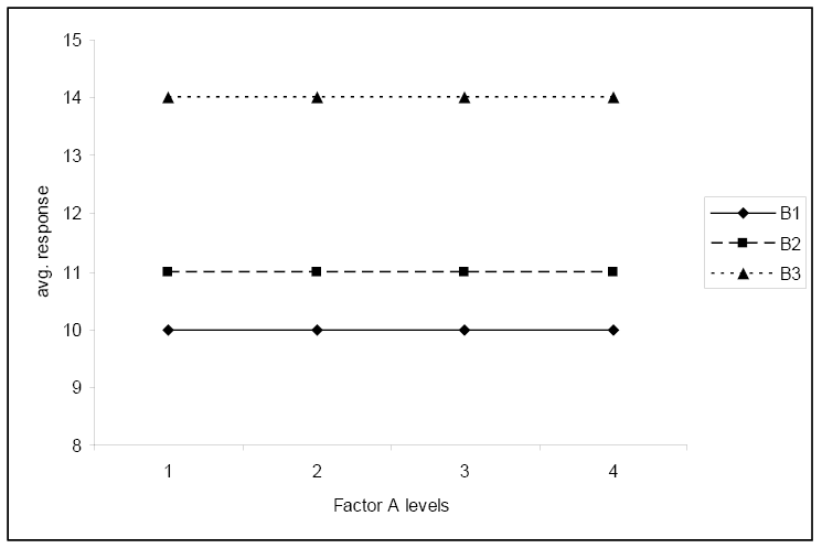
The third plot shows no significant interaction and shows that the average response does not depend on the level of factor A.
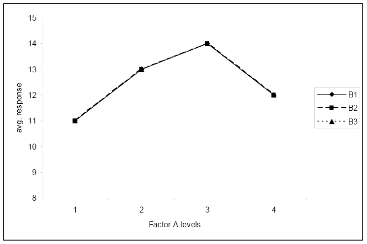
This fourth plot again shows no significant interaction and shows that the average response does not depend on the level of factor B.
This final plot illustrates no interaction and neither factor has any effect on the response.